graph representation learning and its applications a survey

An official website of the United States government

The .gov means it’s official. Federal government websites often end in .gov or .mil. Before sharing sensitive information, make sure you’re on a federal government site.

The site is secure. The https:// ensures that you are connecting to the official website and that any information you provide is encrypted and transmitted securely.

Publications
Account settings
My Bibliography
Collections
Citation manager

Save citation to file

Email citation, add to collections.

Create a new collection
Add to an existing collection

Add to My Bibliography

Your saved search, create a file for external citation management software, your rss feed.

Search in PubMed
Search in NLM Catalog
Add to Search

Graph Representation Learning and Its Applications: A Survey

Affiliations.

1 Department of Artificial Intelligence, The Catholic University of Korea, 43, Jibong-ro, Bucheon-si 14662, Gyeonggi-do, Republic of Korea.
2 Data Assimilation Group, Korea Institute of Atmospheric Prediction Systems (KIAPS), 35, Boramae-ro 5-gil, Dongjak-gu, Seoul 07071, Republic of Korea.
3 Department of Social Welfare, Dongguk University, 30, Pildong-ro 1-gil, Jung-gu, Seoul 04620, Republic of Korea.
4 Semiconductor Devices and Circuits Laboratory, Advanced Institute of Convergence Technology (AICT), Seoul National University, 145, Gwanggyo-ro, Yeongtong-gu, Suwon-si 16229, Gyeonggi-do, Republic of Korea.
PMID: 37112507
PMCID: PMC10144941
DOI: 10.3390/s23084168

Graphs are data structures that effectively represent relational data in the real world. Graph representation learning is a significant task since it could facilitate various downstream tasks, such as node classification, link prediction, etc. Graph representation learning aims to map graph entities to low-dimensional vectors while preserving graph structure and entity relationships. Over the decades, many models have been proposed for graph representation learning. This paper aims to show a comprehensive picture of graph representation learning models, including traditional and state-of-the-art models on various graphs in different geometric spaces. First, we begin with five types of graph embedding models: graph kernels, matrix factorization models, shallow models, deep-learning models, and non-Euclidean models. In addition, we also discuss graph transformer models and Gaussian embedding models. Second, we present practical applications of graph embedding models, from constructing graphs for specific domains to applying models to solve tasks. Finally, we discuss challenges for existing models and future research directions in detail. As a result, this paper provides a structured overview of the diversity of graph embedding models.

Keywords: graph embedding; graph neural networks; graph representation learning; graph transformer.

PubMed Disclaimer

Conflict of interest statement

The authors declare no conflict of interest.

The popularity of graph representation…

The popularity of graph representation learning models in the Scopus database. The line…

A comprehensive view of graph…

A comprehensive view of graph embedding. Given a spare, high-dimensional graph G =…

Methods for modeling dynamic graphs…

Methods for modeling dynamic graphs over time. ( a ) The representation of…

The proposed taxonomy for graph…

The proposed taxonomy for graph representation learning models.

The Weisfeiler–Lehman isomorphism test. (…

The Weisfeiler–Lehman isomorphism test. ( a ) Original labels, i = 0 ;…

Node sampling techniques. ( a…

Node sampling techniques. ( a ) k -hop sampling; ( b ) Random-walk…

Sampling strategy in Node2Vec and…

Sampling strategy in Node2Vec and WalkLets model. ( a ) Sampling strategy in…

Sampling strategy in Sub2Vec model.…

Sampling strategy in Sub2Vec model. Assume that there are two subgraphs G 1…

The random-walk sampling based on…

The random-walk sampling based on motif. ( a ) Random-walk sampling; ( b…

Updating random-walk paths to the…

Updating random-walk paths to the corpus on dynamic graphs. At time t ,…

The strategy of edge and…

The strategy of edge and node collapsing of HARP model. ( a )…

The self-centered network of NEWEE…

The self-centered network of NEWEE model. For instance, the self-centered of node v…

The architecture of SDNE model.…

The architecture of SDNE model. The features of nodes x i and x…

The architecture of DynGEM model.…

The architecture of DynGEM model. Similarity to the SDNE model, the DynGEM model…

An example of the Topo-LSTM…

An example of the Topo-LSTM model. Given by a cascade sequence S =…

The sampling strategy of [57].…

The sampling strategy of [57]. The model lists all the node pairs in…

The temporal random-walk sampling strategy…

The temporal random-walk sampling strategy of LSTM-Node2Vec model during the graphs’ evolution. (…

An example of the GraphSAINT…

An example of the GraphSAINT model. ( a ) A subgraph has five…

The architecture of GAE and…

The architecture of GAE and VGAE model. The model adopts the adjacency matrix…

Publication types

Search in MeSH

Grants and funding

2022R1F1A1065516/National Research Foundation of Korea
KMA2020-02211/Korea Meteorological Administration
2022M3F3A2A01076569/National Research Foundation of Korea
AICT-2022-0015/Advanced Institute of Convergence Technology
M-2022-B0008-00153/The Catholic University of Korea

LinkOut - more resources

Full text sources.

Europe PubMed Central
PubMed Central

Research Materials

NCI CPTC Antibody Characterization Program

Citation Manager

NCBI Literature Resources

MeSH PMC Bookshelf Disclaimer

The PubMed wordmark and PubMed logo are registered trademarks of the U.S. Department of Health and Human Services (HHS). Unauthorized use of these marks is strictly prohibited.

Europe PMC requires Javascript to function effectively.

Either your web browser doesn't support Javascript or it is currently turned off. In the latter case, please turn on Javascript support in your web browser and reload this page.

IEEE Account

Change Username/Password
Update Address

Purchase Details

Payment Options
Order History
View Purchased Documents

Profile Information

Communications Preferences
Profession and Education
Technical Interests
US & Canada: +1 800 678 4333
Worldwide: +1 732 981 0060
Contact & Support
About IEEE Xplore
Accessibility
Terms of Use
Nondiscrimination Policy
Privacy & Opting Out of Cookies

A not-for-profit organization, IEEE is the world's largest technical professional organization dedicated to advancing technology for the benefit of humanity. © Copyright 2024 IEEE - All rights reserved. Use of this web site signifies your agreement to the terms and conditions.

Export citation

Select the format to use for exporting the citation.

Graph representation learning: a survey

Journal details.

This is published under the terms of the Creative Commons Attribution licence.

Downloaded: 6990 times

I. INTRODUCTION
II. DEFINITION AND PRELIMINARIES
III. Graph embedding methods
IV. COMPARISON OF DIFFERENT METHODS and APPLICATIONS
V. EVALUATION
VI. EMERGING APPLICATIONS
VII. FUTURE RESEARCH DIRECTIONS
VIII. CONCLUSION

Research on graph representation learning has received great attention in recent years since most data in real-world applications come in the form of graphs. High-dimensional graph data are often in irregular forms. They are more difficult to analyze than image/video/audio data defined on regular lattices. Various graph embedding techniques have been developed to convert the raw graph data into a low-dimensional vector representation while preserving the intrinsic graph properties. In this review, we first explain the graph embedding task and its challenges. Next, we review a wide range of graph embedding techniques with insights. Then, we evaluate several stat-of-the-art methods against small and large data sets and compare their performance. Finally, potential applications and future directions are presented.

An official website of the United States government

The .gov means it’s official. Federal government websites often end in .gov or .mil. Before sharing sensitive information, make sure you’re on a federal government site.

The site is secure. The https:// ensures that you are connecting to the official website and that any information you provide is encrypted and transmitted securely.

Publications
Account settings

Preview improvements coming to the PMC website in October 2024. Learn More or Try it out now .

Advanced Search
Journal List
Sensors (Basel)
PMC10144941

Graph Representation Learning and Its Applications: A Survey

Van thuy hoang.

1 Department of Artificial Intelligence, The Catholic University of Korea, 43, Jibong-ro, Bucheon-si 14662, Gyeonggi-do, Republic of Korea; moc.liamg@09yuhtnavgnaoh (V.T.H.); moc.revan@ereinset (E.-S.Y.)

Hyeon-Ju Jeon

2 Data Assimilation Group, Korea Institute of Atmospheric Prediction Systems (KIAPS), 35, Boramae-ro 5-gil, Dongjak-gu, Seoul 07071, Republic of Korea; gro.spaik@noejjh

Eun-Soon You

Yoewon yoon.

3 Department of Social Welfare, Dongguk University, 30, Pildong-ro 1-gil, Jung-gu, Seoul 04620, Republic of Korea; ude.kuggnod@nooyy

Sungyeop Jung

4 Semiconductor Devices and Circuits Laboratory, Advanced Institute of Convergence Technology (AICT), Seoul National University, 145, Gwanggyo-ro, Yeongtong-gu, Suwon-si 16229, Gyeonggi-do, Republic of Korea; [email protected]

Associated Data

Data sharing not applicable.

1. Introduction

Graphs are a common language for representing complex relational data, including social media, transportation system networks, and biological protein–protein networks [ 1 , 2 ]. Since most graph data are complex and high-dimensional, it is difficult for researchers to extract valuable knowledge. Therefore, processing graph data and transforming them into a form (fixed-dimensional vectors) is an important process that researchers can then apply to different downstream tasks [ 3 ]. The objective of graph representation learning is to obtain vector representations of graph entities (e.g., nodes, edges, subgraphs, etc.) to facilitate various downstream tasks, such as node classification [ 4 ], link prediction [ 5 , 6 ], community detection [ 7 ], etc. As a result, graph representation learning plays an important role since it could significantly promote the performance of the downstream tasks.

Representation of the graph data, however, is challenging and different from image and text data [ 8 ]. In textual data, words are linked together in a sentence, and they have a fixed position in that sentence. In image data, pixels are arranged on an ordered grid space and can be represented by a grid matrix. However, the nodes and edges in graphs are non-ordered and have their features. This leads to mapping graph entities to latent space while preserving the graph structure, and proximity relationships are challenging. In the case of a social network, a user can have many friends (neighbors) and various personal information, such as hometown, education level, and hobbies, which makes preserving the graph structure and properties significantly problematic. In addition, many real-world networks show dynamic behaviors in which graph structures and node features could be changed over time [ 9 , 10 ]. These could deliver challenges in capturing the graph structure and mapping graph entities into vector space.

Over decades, various graph representation learning models have been proposed to project graph entities into fixed-length vectors [ 11 , 12 , 13 ]. Graph embedding models are mainly divided into five main groups: graph kernels, matrix factorization models, shallow models, deep neural network models, and non-Euclidean models. Figure 1 presents the popularity of different graph representation learning models from 2010 to 2022. The number of graph representation learning studies increased considerably over the period of 12 years. Furthermore, there was significant growth in the frequency of research studies on graph neural networks, graph convolutional networks, and graph transformer models. In contrast, the number of studies in graph kernels, graph autoencoder, and matrix factorization-based models increased slightly over the period of 12 years. We obtained the frequency of academic publications including each keyword from Scopus ( https://www.scopus.com (accessed on 16 April 2023)).

An external file that holds a picture, illustration, etc.
Object name is sensors-23-04168-g001.jpg

The popularity of graph representation learning models in the Scopus database. The line plot shows changes in the number of publications in different types of graph representation learning models from 2010 to 2022. The y-axis denotes the number of publications on the popularity of graph representation learning models over the years. There are seven keywords, including graph representation learning (GRL), graph kernels (GK), matrix factorization-based graph embedding (MF), graph neural networks (GNNs), graph autoencoder (GAE), graph convolution networks (GCNs), graph transformer (GT), and non-Euclidean graph embedding (NEGE). There are nineteen representative models, including DeepWalk [ 14 ], Grarep [ 15 ], LINE [ 16 ], GGCN [ 17 ], GCN [ 18 ], HOPE [ 5 ], Node2Vec [ 4 ], GAT [ 19 ], Metapath2Vec [ 20 ], Struc2Vec [ 21 ], GraphSage [ 22 ], G2G [ 23 ], GIN [ 24 ], HGAT [ 25 ], DGI [ 26 ], HGNN [ 27 ], GCNII [ 28 ], GT [ 29 ], and EGT [ 30 ].

Historically, the first graph representation learning models were graph kernels. The idea of graph kernel methods perhaps comes from the most essential and well-known Weisfeiler–Lehman (WL) isomorphic testing in 1968 [ 31 ]. Graph kernels are kernel functions that aim to measure the similarity between graphs and their entities [ 32 ]. The main idea of graph kernels is to decompose original graphs into substructures and construct vector embeddings based on the substructure features. There are two main types of graph kernels: kernels for graphs and kernels on graphs. The former aims to measure the similarity between pairs of graphs, while the latter estimates the similarity between graph nodes. Several strategies to estimate the similarity of graph pairs have been proposed to represent various graph structures, such as graphlet kernels, random walk, and the shortest path, which started in the 2000s. Based on WL isomorphic testing, various graph kernels are built to compute the similarity of pairs of graph entities, such as WL kernels [ 31 ], WL subtree kernels [ 33 , 34 , 35 ], and random walks [ 36 , 37 ]. However, one of the limitations of graph kernels is the computational complexity when working with large-scale graphs since computing graph kernels is an NP-hard class.

Early models for graph representation learning primarily focused on matrix factorization methods, which are motivated by traditional techniques for dimensionality reduction in 2002 [ 38 ]. Several matrix factorization-based models have been proposed to handle large graphs with millions of nodes [ 39 , 40 ]. The objective of matrix factorization models is to decompose the proximity matrix into a product of small-sized matrices and then learn the embeddings that fit the proximity. Based on the ways to learn vector embeddings, there are two main lines of matrix factorization models: Laplacian eigenmaps and node proximity matrix factorization. Starting in the 2000s, Laplacian eigenmaps methods [ 41 , 42 ] aim to represent each node by Laplacian eigenvectors along with the first k eigenvalues. In contrast, the node proximity matrix factorization methods [ 5 , 15 ] aim to gain node embeddings by the singular value decomposition in 2015. Various proximity matrix factorization models have successfully handled large graphs and achieved great performance [ 15 , 43 ]. However, matrix factorization models suffer from capturing high-order proximity due to computational complexity when performing with high transition matrices.

In 2014 and 2016, early shallow models, DeepWalk [ 14 ] and Node2Vec [ 4 ] were proposed, which learn node embeddings based on shallow neural networks. Remarkably, the primary concept is to learn node embeddings by maximizing the neighborhood probability of target nodes using the skip-gram model started in the natural language processing area. The purpose of this strategy could then be optimized with SGD on neural network layers, thus reducing computational complexity. With this historic milestone, various models have been developed by improving multiple sampling strategies and training processes. Shallow models are the embedding models that aim to map graph entities to low-dimensional vectors by conducting an embedding lookup for each graph entity [ 3 ]. From this perspective, the embedding of node v i could be represented as Z i = M x i , where M denotes an embedding matrix of all nodes and x i is a one-hot vector of node v i . Various shallow models have been proposed to learn embeddings with different strategies to preserve graph structures and the similarity between graph entities. Structure-preservation models aim to preserve the structural connection between entities (e.g., DeepWalk [ 14 ], Node2Vec [ 4 ]). In 2015, Tang et al. [ 16 ] proposed the LINE model, a proximity reconstruction method that aims to preserve proximity between nodes in graphs. After that, various models have been proposed to preserve the node proximity with higher-order proximity and capture more global graph structure. However, most of the above models focus on transductive learning and ignore node features, which may have several limitations to practical applications.

Breakthroughs in deep learning have led to a new research perspective on applying deep neural networks to the graph domain. Since the 2000s, there have been several early models on GNNs designed to learn node embeddings based on neighborhood information using an aggregation mechanism [ 44 , 45 ]. Graph neural networks (GNNs) have shown a significant expressive capacity to represent graph embeddings in an inductive learning manner and solve the limitations of aforementioned shallow models [ 46 , 47 ]. Recurrent GNNs are also the first studies on GNNs based on recurrent neural network architecture [ 48 , 49 ] in 2005. These models aim to learn node embeddings via recurrent layers with the same weights in each hidden layer and run recursively until convergence. Several recurrent GNNs with different strategies have been proposed by the power of recurrent neural network architecture and the combinations with several sampling strategies. However, using the same weights at each hidden layer of the RGNN model may cause the model to be incapable of distinguishing the local and global structure. Since 2016, several graph autoencoder models have been proposed based on the original autoencoder architecture, which could learn complex graph structures by reconstructing the input graph structure [ 50 , 51 ]. The graph autoencoders comprise two main layers: encoder layers take the adjacency matrix as input and squeeze it to generate node embeddings, and decoder layers reconstruct the input data. By contrast, the idea of CGNNs is to use convolutional operators with different weights in each hidden layer, which are more efficient in capturing and distinguishing the local and global structures [ 18 , 52 , 53 , 54 ]. Many studies have been proposed with various variants of CGNNs, including spectral CGNNs [ 55 , 56 , 57 ] started in 2014, spatial CGNNs [ 22 , 24 , 52 ] started in 2016, and attentive CGNNs [ 19 , 58 ] started in 2017. Nevertheless, most GNNs suffer limitations such as over-smoothing problems and noise from neighbor nodes when stacking more GNN layers [ 59 , 60 ].

Motivated by transformer architecture started from natural language processing applications in 2017, several graph transformer models were proposed using the transformer architecture to the graph domain in 2019 [ 61 , 62 ]. Graph transformer models have shown competitive and superior performance against GNNs in learning complex graph structures [ 30 , 63 ]. Graph transformer models can be divided into three main groups: transformer for tree-like graphs, transformer with GNNs, and transformer with global self-attention. Early graph transformer models aim to learn tree-like graphs, which mainly aim at learning node embeddings in tree-like graphs where nodes are arranged hierarchically [ 64 , 65 ] since 2019. These models encode the node positions through their relative and absolute positional encoding in trees as constraints with root nodes and neighbor nodes at the same level. Second, several models leverage the power of GNNs as an auxiliary module in computing attention scores [ 66 ]. In addition, some models put GNN layers on top of the model to overcome the over-smoothing problem and make the model remember the local structure [ 61 ]. Most above graph transformer models adopt vanilla transformer architecture to learn embeddings that rely on multi-head self-attention. Third, several graph transformer models use a global self-attention mechanism to learn node embeddings, which implements self-attention independently and does not require constraints from the neighborhood [ 30 , 67 ]. These models work directly on input graphs and can capture the global structure with global self-attention.

Most of the above models learn embeddings in Euclidean space and represent graph entities as vector points in latent space. However, graphs in the real world could have complex structures and different forms, such that Euclidean space may be inadequate to represent the graph structure and ultimately lead to structural loss [ 68 , 69 ]. Early models learn complex graphs in non-Euclidean geometry by developing efficient algorithms for learning node embeddings based on manifold optimization [ 70 ] in 2017. Following the line, several models aim to represent graph data in non-Euclidean space and gain desirable results [ 68 , 69 , 71 ]. Two typical non-Euclidean spaces, including spherical and hyperbolic geometry, have their advantages. Spherical space could represent graph structures with large cycles, while hyperbolic space is suitable for hierarchical graph structures. Most non-Euclidean models aim to design an efficient algorithm for learning node embeddings since it is challenging to implement operators directly in non-Euclidean. Furthermore, to deal with uncertainty, several Gaussian graph models have been introduced to represent graph entities as density-based embeddings [ 23 ] started in 2016. Node embeddings could be defined as a continuous density mostly based on Gaussian distribution [ 72 ].

To the extent of our knowledge, no comparable paper in the literature focuses on a wide range of graph embedding models for static and dynamic graphs in different geometric spaces. Most current papers only presented specific approaches for graph representation learning. Wu et al. [ 8 ] focused on graph neural network models, which are presented as a section in this paper. Several surveys [ 13 , 73 , 74 ] summarized graph embedding models for various types of graphs, but they did not mention either graph transformer models or non-Euclidean models. From applying graph embedding models to practical applications, several papers only list the applications for specific and narrow tasks [ 12 , 75 ]. However, we discuss how graphs are constructed in specific applications and how graph embedding models are implemented in various domains.

This paper presents a comprehensive picture of graph embedding models in static and dynamic graphs in different geometric spaces. In particular, we recognize five general categories of models for addressing graph representation learning, including graph kernels, matrix factorization models, shallow models, deep neural network models, and non-Euclidean models. The contribution of this study can be categorized as follows:

This paper presents a taxonomy of graph embedding models based on various algorithms and strategies.
We provide readers with an in-depth analysis of an overview of graph embedding models with different types of graphs ranging from static to dynamic and from homogeneous to heterogeneous graphs.
This paper presents graph transformer models, which have achieved remarkable results in a deeper understanding of graph structures in recent years.
We cover applications of graph representation learning in various areas, from constructing graphs to applying models in specific tasks.
We discuss the challenges and future directions of existing graph embedding models in detail.

Since abundant graph representation learning models have been proposed recently, we employed different approaches to find related studies. We built a search strategy by defining keywords and analyzing reliable sources. The list of keywords includes graph embedding, graph representation learning, graph neural networks, graph convolution, graph attention, graph transformer, graph embedding in non-Euclidean space, Gaussian graph embedding, and applications of graph embedding. We found related studies at famous top-tier conferences and journals such as AAAI, IJCAI, SIGKDD, ICML, WSDM, Nature Machine Intelligence, Pattern Recognition, Intelligent Systems with Applications, the Web, and so on.

The following sections of this paper are summarized as follows. Section 2 describes fundamental concepts and backgrounds related to graph representation learning. In Section 3 , all the graph embedding models will be presented, such as graph kernels, matrix factorization models, shallow models, deep neural network models, and non-Euclidean models. Section 4 discusses a wide range of practical applications of graph embedding models in the real world. Section 5 summarizes the latest benchmarks, downstream tasks, evaluation metrics, and libraries. Challenges for existing graph embedding models and future research directions will be discussed in Section 6 . The last section, Section 7 is the conclusion.

2. Problem Description

Graph representation learning aims to project the graph entities into low-dimensional vectors while preserving the graph structure and the proximity of entities in graphs. With the desire to map graph entities into vector space, it is necessary to model the graph in mathematical form. Therefore, we begin with several fundamental definitions of graphs. The list of standard notations used in this survey is detailed in Table 1 . Mathematically, a graph G can be defined as follows:

A summary of notations.

Notations	Descriptions
	The set of nodes in the graph
	The set of edges in graph
	The number of nodes in graph
	The set of edges with type in heterogeneous graphs
	The node in the graph
	The edge in the graph
	The adjacency matrix of the graph
	The feature matrix of nodes in graph
	The degree matrix of nodes in graph
	Projection function
	The embedding vector of node
	The transition matrix
	The set of neighbors of node
	The -hop distance from a target node to other nodes
	The dimension of vector in latent space
	The label of node

(Graph [ 3 ]). A graph is a discrete structure consisting of a set of nodes and the edges connecting those nodes. The graph can be described mathematically in the form: G = ( V , E , A ) , where V = { v 1 , v 2 , ⋯ , v N } is the set of nodes, E = { ( v i , v j ) | ( v i , v j ) ∈ V × V } is the set of edges, and A is an adjacency matrix. A is a square matrix of size N × N where N is the number of nodes in graphs. This can be formulated as follows:

where A i j indicates adjacency between node v i and node v j .

When A i j is binary, the matrix A represents only the existence of connections between nodes. By extending the definition of matrix A , we could expand to abundant different types of graph G :

Directed graph: When A i j = A j i for any 1 ≤ i , j ≤ n , then the graph G is called an undirected graph, and G is directed graph otherwise.
Weighted graph: is a graph in which each edge is assigned a specific weight value. Therefore, the adjacency matrix could be presented as: A i j = w i j , where w i j ∈ R is the weight of the edge e i j .
Signed graph: When A i j ∈ [ − ∞ , ∞ ] , the graph G is called signature/signed graph. The graph G could have all positive signed edges when A i j > 0 for any 1 ≤ i , j ≤ n , and G could have all negative signed edges otherwise.
Attributed graph: A graph G = ( V , E , A , X ) is an attributed graph where V , E is the set of nodes and edges, respectively, and X is the matrix of node attributes with size n × d . Furthermore, we could also have the matrix X as the matrix of edge input attribute with size m × d where m is the number of edges e i j ∈ E for any 1 ≤ i , j ≤ n .
Hyper graph: A hyper graph G could be represented as G = ( V , E , W ) , where V denotes the set of nodes and E denotes a set of hyperedge. Each hyperedge e i j can connect multiple nodes and is assigned a weight w i j ∈ W . The hypergraph G could be represented by an incidence matrix H size V × E with entries h ( v i , v j ) = 1 if e i j ∈ E , and h ( v i , v j ) = 0 otherwise.
Heterogeneous graph: A heterogeneous graph is defined as G = ( V , E , T , φ , ρ ) where V , and E are the set of nodes and edges, respectively, φ is the mapping function: φ : V → T v , and the mapping function ρ : E → T e with T v , T e describe the set of node types and edge types, respectively, and T = T v + T e is the sum of the number of node types and edge types.

According to the definitions of graph G = ( V , E ) that have been represented mathematically above, the idea of graph embedding is to map graph entities into low-dimensional vectors with the number of dimensions d with d ≪ N . Mathematically, the graph embedding is formulated as follows:

(Graph embedding [ 14 ]). Given a graph G = ( V , E ) where V is the set of nodes, and E is the set of edges, graph embedding is a projection function ϕ ( · ) , where ϕ : V → R d ( d ≪ | V | ) and k ( v i , v j ) ≃ 〈 ϕ ( v i ) , ϕ ( v j ) 〉 describes the proximity of two nodes v i and v j in the graph and 〈 ϕ ( v i ) , ϕ ( v j ) 〉 is the distance of two vectors ϕ ( v i ) and ϕ ( v j ) in the vector space.

Graph representation learning aims to project graph entities into the vector space while preserving the graph structure and entity proximity. For example, if two nodes v i and v j in the graph G are connected directly, then in vector space, the distance between two vectors ϕ ( v i ) and ϕ ( v j ) must be minimal. Figure 2 shows an example of a graph embedding model that transforms nodes in a graph to low-dimensional vectors ( Z 1 Z 2 ⋯ Z n ) in the vector space.

An external file that holds a picture, illustration, etc.
Object name is sensors-23-04168-g002.jpg

A comprehensive view of graph embedding. Given a spare, high-dimensional graph G = ( V , E ) where V and E denote the set of nodes and edges. Graph embedding learning aims to find a function ϕ that maps nodes from graph space to d -dimensional vector space with d ≪ | V | .

When mapping graph entities to latent space, preserving the proximity of graph entities is one of the most important factors in preserving the graph structure and the relationship between nodes. In other words, if two nodes v i and v j are connected or close in the graph, the distance between the two vectors Z i and Z j must be minimal in the vector space. Several models [ 16 , 76 , 77 , 78 ] aim to preserve k -order proximity between graph entities in vector space. Formally, the k -order proximity is defined as follows:

( k -order proximity [ 79 ]). Given a graph G = ( V , E ) where V is the set of nodes, and E is the set of edges, k-order proximity describes the similarity of nodes with the distance captured from the k-hop in the graph G. When k = 1 , it is 1st-order proximity that captures the local pairwise proximity of two nodes in graphs. When k is higher, it could capture the global graph structure.

There is another way to define graph embedding from the perspective of Encoder-Decoder architecture [ 3 ]. From this perspective, the task of the encoder part is to encode graph entities into low-dimensional vectors, and the decoder part tries to reconstruct the graph from the latent space. In the real world, many graphs show dynamic behaviors, including node and edge evolution, and feature evolution [ 80 ]. Dynamic graphs are found widely in many applications [ 81 ], such as social networks where connections between friends could be added or removed over time.

(Dynamic graph [ 80 ]). A dynamic graph G is formed of three entities: G = V , E , T where V = V t is the group of node sets, E = { E ( t ) } with t ∈ T is the group of edge sets over time span T, and T denotes the time span. From the statistic perspective, we could also consider a dynamic graph G = { G ( t 0 ) G ( t 1 ) ⋯ G ( t n ) } as a collection of static graphs G ( t k ) where G ( t k ) = V ( t k ) , E ( t k ) denotes the static graph G at time t k , and V ( t k ) , E ( t k ) denotes the set of nodes and set of edges at time t k , respectively.

Figure 3 a presents an example of dynamic graph representation. At time t + 1 , there are several changes in the graph G ( t + 1 ) such as: The edge e 23 will be removed, node v 6 will be added and new edge e 56 . Casteigts et al. [ 80 ] proposed an alternative definition of a dynamic graph with five components: G = ( V , E , T , ρ , ζ ) where ρ : V × T → { 0 , 1 } describes the existence of each node at time t , and ζ : E × T → Ψ describes the existence of an edge at time t .

An external file that holds a picture, illustration, etc.
Object name is sensors-23-04168-g003.jpg

Methods for modeling dynamic graphs over time. ( a ) The representation of a dynamic graph by a series of snapshots; ( b ) The evolution of edges and nodes in the dynamic graph from time t to t + 1 . In ( a ), the graph G is the collection of G ( t ) (i.e., G = { G ( 1 ) , G ( 2 ) , ⋯ , G ( t ) } ) which t is the time span, and the entities of G change from time t to t + 1 . ( b ) depicts the evolution of edges in the same dynamic graph from ( a ) which each edge contains the series of the time spans from t to t + 1 . At time t , the graph has five nodes ( v 1 , v 2 , v 3 , v 4 , v 5 ) and five edges ( e 13 e 15 e 34 e 45 e 23 ) . However, at time t + 1 , the edge e 23 and node v 2 are removed, and a new node v 6 , a new edge e 56 are added in the graph.

There is another way to model a dynamic graph based on the changes of the graph entities (edges, nodes) taking place on the graph G over a time span t or by an edge stream. From this perspective, a dynamic G could be modeled as G = ( V , E t , T ) where E t presents the collection of edges of dynamic graph G at time t , and function f : E → R + to map edges into integer numbers. It notices that all the edges at time t will have the same labels. Figure 3 b describes the evolution of the edges of a graph from time ( t ) to ( t + 1 ) .

(Dynamic graph embedding [ 82 ]). Given a dynamic graph G = ( V , E , T ) where V = { V ( t ) } is the group of node sets, and E = { E ( t ) } is the group of edge sets over time span T, a dynamic graph embedding is a projection function ϕ ( · ) , where ϕ ( · ) : G × T → R d × T . T describes the time domain in latent space and T is the time span. When G is represented as the collection of snapshots: G = { G ( t 0 ) G ( t 1 ) ⋯ G ( t n ) } , then the projection function ϕ will be defined as: ϕ = { ϕ ( 0 ) ϕ ( 1 ) ⋯ ϕ ( n ) } where ϕ ( t ) is the vector embedding of the graph G ( t ) at time t.

There are two ways to represent a dynamic graph G , including a temporal dynamic graph embedding (changes over a period of time) and topological dynamic graph embedding (changes in the graph structure over time).

Temporal dynamic graph embedding: A temporal dynamic embedding is a projection function ϕ ( · ) , where ϕ t : G t − k , t × T → R d × T and G t − k , t = { G t − k G t − k + 1 ⋯ G t } describes the collection of graph G during time interval [ t − k , t ] .
Topological dynamic graph embedding: A topological dynamic graph embedding for graph G for nodes is a mapping function ϕ , where ϕ : V × T → R d × T .

3. Graph Representation Learning Models

This section presents a taxonomy of existing graph representation learning models in the literature. We categorize the existing graph embedding models into five main groups based on strategies to preserve graph structures and proximity of entities in graphs, including graph kernels, matrix factorization-based models, shallow models, deep neural network models, and non-Euclidean models. Figure 4 presents the proposed taxonomy of the graph representation learning models. Furthermore, we deliver open-source implementations of graph embedding models in Appendix A .

An external file that holds a picture, illustration, etc.
Object name is sensors-23-04168-g004.jpg

The proposed taxonomy for graph representation learning models.

Graph kernels and matrix factorization-based models are one of the pioneer models for graph representation learning. Graph kernels are prevalent in learning graph embeddings using a deterministic mapping function in solving graph classification tasks [ 83 , 84 , 85 ]. There are two types of graph kernels: kernels for graphs, which aim to compare the similarity between graphs, and kernels on graphs aim to find the similarity between nodes in graphs. Second, matrix factorization-based models aim to represent the graph as matrices and gain embeddings by decomposing the matrices [ 5 , 86 ]. There are several strategies for factorization modeling, and most of these models aim to approximate high-order proximity between nodes. However, graph kernels and matrix factorization-based models suffer from computational complexity when handling large graphs and capturing high-order proximity.

Shallow models aim to construct an embedding matrix to transform each graph entity into vectors. We categorize shallow models into two main groups: structure preservation and proximity reconstruction. Structure-preservation strategies aim to conserve structural relationships between nodes in graphs [ 4 , 14 , 87 ]. Depending on specific tasks, several sampling strategies could be employed to capture graph structures, such as random walks [ 4 , 14 ], graphlets [ 88 ], motifs [ 89 , 90 , 91 ], etc. By contrast, the objective of the proximity reconstruction models is to preserve the proximity of nodes in graphs [ 16 , 92 ]. The proximity strategies can vary across different models based on their objectives. For example, the LINE model [ 16 ] aims to preserve 1st-order and 2nd-order proximity between nodes, while PALE [ 77 ] preserves pairwise similarities.

Graph neural networks have shown great performance in learning complex graph structures [ 18 , 50 ]. GNNs can be categorized into three main groups: graph autoencoder [ 50 , 51 ], recurrent GNNs [ 17 , 93 ], and convolutional GNNs. Graph autoencoders and recurrent GNNs are mostly pioneer studies of GNNs based on autoencoder architecture and recurrent neural networks, respectively. Graph autoencoders are composed of an encoder layer and a decoder layer. The encoder layer aims to compress a proximity graph matrix to vector embeddings, and the decoder layer reconstructs the proximity matrix. Most graph autoencoder models employ multilayer perceptron-based layers or recurrent GNNs as the core of autoencoder architecture. Recurrent GNNs aim to learn node embeddings based on recurrent neural network architecture in which connections between neurons can make a cycle. Therefore, earlier RGNNs mainly aimed to learn embeddings on directed acyclic graphs [ 94 ]. Recurrent GNNs employ the same weights in all hidden layers to capture local and global structures. Recently, convolutional GNNs have been much more efficient and can gain outstanding performance compared to RGNNs. The main difference between RGNNs and CGNNs is that CGNNs use different weights in each hidden layer, which could distinguish local and global structures. Various CGNN models have been proposed and mainly fall into two categories: spectral CGNNs, and spatial CGNNs [ 22 , 52 , 95 ]. Spectral CGNNs aim to transform graph data to the frequency domain and learn node embeddings in this domain [ 56 , 96 ]. By contrast, spatial CGNNs work directly on the graph using convolutional filters [ 53 , 54 ]. By staking multiple GNN layers, the models could learn node embeddings more efficiently and capture higher-order structural information [ 97 , 98 ]. However, stacking many layers could cause the over-smoothing problem, which most GNNs have not fully solved in a whole extent.

Recently, several models have enabled transformer architecture to learn graph structures which gain significant results compared to other deep-learning models [ 30 , 46 , 99 ]. We categorize graph transformer models into three main groups: transformer for tree-like graphs [ 64 , 65 ], transformer with GNNs [ 99 , 100 ], and transformer with global self-attention [ 30 , 67 ]. Different types of graph transformer models aim to handle distinct types of graphs. The transformer for tree-like graphs aims to learn node embeddings in tree-like hierarchical graphs [ 64 , 65 , 101 ]. The hierarchical relationships from the target nodes to their parents and neighbors are presented as absolute and relative positional encoding, respectively. Several graph transformer models employ the message-passing mechanism from GNNs as an auxiliary module in computing the attention score matrix [ 61 , 100 ]. GNN layers can be used to aggregate information as input to graph transformer models or put on top of the model, which aims to preserve local structures. In addition, some graph transformer models can directly process graph data without support from GNN layers [ 30 , 67 ]. These models implement a global self-attention to learn local and global structures in a graph input without neighborhood constraints.

Most existing graph embedding models aim to learn embeddings in Euclidean space, which may not deliver good geometric representations and metrics. Recent studies have shown that non-Euclidean spaces are more suitable for representing complex graph structures. The non-Euclidean models could be categorized as hyperbolic, spherical, and Gaussian. Hyperbolic and spherical space are two types of non-Euclidean geometry that could represent different graph structures. Hyperbolic space [ 102 ] is more suitable for representing hierarchical graph structures that follow the power law, while the power of spherical space is to represent large circular graph structures [ 103 ]. Moreover, since the information about the embedding space is unknown and uncertain, several models aim at learning node embeddings as Gaussian distribution [ 23 , 104 ].

3.1. Graph Kernels

Graph kernels aim to compare graphs or their substructures (e.g., nodes, subgraphs, and edges) by measuring their similarity [ 105 ]. The problem of measuring the similarity of graphs is, therefore, at the core of learning graphs in an unsupervised manner. Measuring the similarity of large graphs is problematic since the graph isomorphism problem is assigned to the NP (nondeterministic polynomial time) class. However, it is an NP-complete for subgraphs isomorphism problem. Table 2 describes a summary of graph kernel models.

A summary of graph kernel models.

Models	Graph Types	Tasks
[ ]	Static graphs	Graph comparison
[ ]	Static graphs	Graph comparison
[ ]	Static graphs	Graph classification
[ ]	Static graphs	Graph classification
[ ]	Static graphs	Graph classification
[ ]	Static graphs	Graph classification
[ ]	Static graphs	Graph comparison
[ ]	Attributed graphs	Graph classification
[ ]	Attributed graphs	Graph classification
[ ]	Attributed graphs	Graph classification
[ ]	Attributed graphs	Graph classification
[ ]	Attributed graphs	Graph classification
[ ]	Attributed graphs	Graph classification
GraTFEL [ ]	Dynamic graphs	Graph reconstruction Link prediction
[ ]	Dynamic graphs	Link prediction
[ ]	Dynamic graphs	Link prediction

Kernel methods applied to the graph embedding problem can be understood in two forms, including the isomorphism testing of N graphs (kernels for graphs) and embedding entities of graphs to Hilbert space (kernels on graphs).

Kernels for graphs: Kernels for graphs aim to measure the similarity between graphs. The similarity between the two graphs (isomorphism) could be explained as follows: Given two undirected graphs G 1 = ( V 1 E 1 ) and G 2 = ( V 2 E 2 ) , G 1 and G 2 are isomorphic if they exist a bimodal mapping function ϕ : V 1 → V 2 such that ∀ a b ∈ V 1 , a and b are contiguous on G 1 if ϕ ( a ) and ϕ ( b ) are contiguous on G 2 .
Kernels on graphs: To embed nodes in graphs, kernel methods refer to finding a function that maps pairs of nodes to latent space using particular similarity measures. Formally, graph kernels could be defined as: Given a graph G = ( V , E ) , a function K = V × V → R is a kernel on G if there is a mapping function ϕ : V → H such that K ( v i v j ) = 〈 ϕ ( v i ) ϕ ( v j ) 〉 for any node pairs ( v i v j ) .

There are several strategies to measure the similarity of pairs of graphs, such as graphlet kernels, WL kernels, random walk, and shortest paths [ 31 , 83 ]. Among the kernel methods, graphlet kernels are one of the simple kernels that could measure the similarity between graphs by counting subgraphs with a limited size k [ 83 , 106 ]. For instance, Shervashidze et al. [ 83 ] introduced a graphlet kernel with the main idea of finding the graph feature by counting the number of different graphlets in graphs. Formally, given an unlabeled graph G , a graphlet list V k = ( G 1 + G 2 + ⋯ + G n k ) is the set of the graphlets with size k where n k depicts the number of graphlets. The graphlet kernel for two unlabeled graphs G and G ′ could be defined as:

where ϕ G and ϕ G ′ are vectors that depict the number of graphlets in a G i and G i ′ , respectively. By counting all graphlets with size k for a graph, the computation time is expensive by the enumeration n k with n depicts the number of nodes in G . One of the practical solutions to overcome this limitation is to design the feature ϕ i G more effectively, called Weisfeiler–Lehman.

Weisfeiler–Lehman (WL) test [ 31 ] is considered to be a traditional strategy to test the homomorphism of two graphs using color refinements. Figure 5 presents the main idea of the WL homomorphism test for two graphs in detail. By updating node labels, all the structure information of nodes in graphs could be stored at each node, including both local and global information, depending on the number of iterations. We can then compute histograms or other summary statistics over these labels as a vector representation for graphs.

An external file that holds a picture, illustration, etc.
Object name is sensors-23-04168-g005.jpg

The Weisfeiler–Lehman isomorphism test. ( a ) Original labels, i = 0 ; ( b ) Relabeled labels, i = 1 . There are two interactions of WL relabeling for the graph with five nodes v 1 , v 2 , v 3 , v 4 , v 5 . In ( a ), labels of nodes are initialized consisting of 5 nodes. In ( b ), in the first iteration, new labels of the nodes will be reassigned and calculated based on the connection information to its adjacent nodes. For example, node v 1 is adjacent to node v 2 and node v 3 , therefore the new label of v 1 is calculated as v 1 , v 2 , v 3 and resigned as new label v 6 . The same steps are repeated until a steady state for the nodes is reached.

Several models improved the idea from WL isomorphism test [ 34 , 84 ]. The concept of the WL isomorphism test inspired various GNN models later, which aim to be expressive as powerful as the WL test to distinguish different graph structures. Shervashidze et al. [ 33 ] presented three instances of WL kernels, including the WL subtree kernel, WL edge kernel, and WL shortest-path kernel with an enrichment strategy for labels. The key idea of [ 33 ] is to represent a graph G as WL sequences with the height of h . The WL sequences of two graphs G and G ′ can be defined as:

where k G i , G i ′ = ϕ ( G i ) , ϕ ( G i ′ ) . For N graphs, the WL subtree kernel could be computed in a runtime of O ( N h m + N 2 h n ) , where h and m are the numbers of interactions and edges in G , respectively. Therefore, the algorithm could capture more information about the graph G after h interactions and compare graphs at different levels.

However, the vanilla WL isomorphism test requires massive resources since the methods are an NP-hard class. Following the WL isomorphism idea, Morris et al. [ 34 ] presented a set of k -set forms V ( G ) k and built a local and global neighborhood of the k -sets. Instead of working on each node in graphs, the models calculate and update the labels based on the k -set. The feature vectors of graph G then could be calculated by counting the number of occurrences of k -sets. Several models [ 84 , 114 ] improved the Wasserstein distance based on the WL isomorphism test, and the models could estimate weights of subtree patterns before the kernel construction [ 35 ]. Several models adopted a random-walk sampling strategy to capture the graph structure that could help reduce the computational complexity to handle large graphs [ 36 , 37 , 85 , 107 ].

However, the above methods only focus on homogeneous graphs in which nodes do not have side information. In the real world, graph nodes could contain labels and attributes and change over time, making it challenging to learn node embeddings. Several models have been proposed with slight variations from the traditional WL isomorphism test and random walk methods [ 109 , 110 , 111 , 112 , 113 ]. For example, Borgwardt et al. [ 109 ] presented random-walk sampling on attributed edges to capture the graph structure. Since existing kernel models primarily work on small-scale graphs or a subset of graphs, improving similarity based on shortest paths could achieve better computational efficiency for graph kernels in polynomial time. An all-paths kernel K could be defined as:

where P ( G 1 ) and P ( G 2 ) are the set of random-walk paths in G 1 and G 2 , respectively, and k p a t h p 1 , p 2 depicts a positive definite kernel on two paths p 1 and p 2 . The model then applied Floyd–Warshall algorithm [ 115 ] to find k shortest-path kernels in graphs. One of the disadvantages of this model is the runtime complexity, which is about O ( k × n 4 ) , where n depicts the number of nodes in graphs. Morris et al. [ 108 ] introduced a variation of the WL subtree kernel for attributed graphs by improving existing shortest-path kernels. The key idea of this model is to use a hash function that maps continuous attributes to label codes, and then it normalizes the discrete label codes.

To sum up, graph kernels are effective models and bring several advantages:

Coverage: The graph kernels are one of the most useful functions to measure the similarity between graph entities by performing several strategies to find a kernel in graphs. This could be seen as a generalization of the traditional statistical methods [ 116 ].
Efficiency: Several kernel tricks have been proposed to reduce the computational cost of kernel methods on graphs [ 117 ]. Kernel tricks could reduce the number of spatial dimensions and computational complexity on substructures while still providing efficient kernels.

Although kernel methods have several advantages, several disadvantages make the kernels difficult to scale:

Missing entities: Most kernel models could not learn node embeddings for new nodes. In the real world, graphs are dynamic, and their entities could evolve. Therefore, the graph kernels must re-learn graphs every time a new node is added, which is time-consuming and difficult to apply in practice.
Dealing with weights: Most graph kernel models do not consider the weighted edges, which could lead to structural information loss. This could reduce the possibility of graph representation in the hidden space.
Computational complexity: Graph kernels are an NP-hard class [ 109 ]. Although several kernel-based models aim to reduce the computational time by considering the distribution of substructures, this may increase the complexity and reduce the ability to capture the global structure.

Although the graph kernels delivered good results when working with small graphs, they remain limitations when working with large and complex graphs [ 118 ]. To address the issue, matrix factorization-based models could bring far more advantages to learning node embeddings by decomposing the large original graphs into small-sized components. Therefore, we discuss matrix factorization-based models for learning node embeddings in the next section.

3.2. Matrix Factorization-Based Models

Matrix factorization aims to reduce the high-dimensional matrix that describes graphs (e.g., adjacency matrix, Laplacian matrix) into a low-dimensional space. Several well-known decomposition models (e.g., SVD, PCA, etc.) are widely applied in graph representation learning and recommendation system problems. Table 3 and Table 4 present matrix factorization-based models for static and dynamic graphs, respectively. Based on the strategy to preserve the graph structures, matrix factorization models could be categorized into two main groups: graph embedding Laplacian eigenmaps and node proximity matrix factorization.

The Laplacian eigenmaps: To learn representations of a graph G = ( V , E ) , these approaches first represent G as a Laplacian matrix L where L = D − A and D is the degree matrix [ 41 ]. In the matrix L , the positive values depict the degree of nodes, and negative values are the weights of the edges. The matrix L could be decomposed to find the smallest number from eigenvalues which are considered node embeddings. The optimal node embedding Z * , therefore, could be computed using an objective function: Z * = arg min Z Z ⊺ L Z . (5)
Node proximity matrix factorization: The objective of these models is to decompose node proximity matrix into small-sized matrices directly. In other words, the proximity of nodes in graphs will be preserved in the latent space. Formally, given a proximity matrix M , the models try to optimize the distance between two pair nodes v i and v j , which could be defined as: Z * = arg min Z M i j − Z i Z j T . (6)

Hofmann et al. [ 119 ] proposed an MSDC (Multidimensional Scaling and Data Clustering) model based on matrix factorization. The key idea of MSDC is to represent data points as a bipartite graph and then learn node embeddings based on node similarity in the graph. This method requires a symmetric proximity matrix M ∈ R N × N as input and learns a latent representation of the data in Euclidean space by minimizing the loss that could be defined as:

However, the limitation of the MSDC model is that the model focuses only on the pairwise nodes, which cannot capture the global graph structure. Furthermore, the model investigated the proximity of all the data points in the graph, which could increase computational complexity when working on large graphs. Several models [ 39 , 120 ] adopted k -nearest methods to search neighbor nodes which can capture more graph structure. The k -nearest methods, therefore, could bring the advantage of reducing computational complexity since the models only take k neighbors as inputs. For example, Han et al. [ 120 ] proposed the similarity S i j between two nodes v i and v j as:

where N k ( v i ) depicts the set of k nearest neighbors of v i in graphs. The model could measure the infringement of the constraints between pairs of nodes regarding label distribution. In addition, the model can estimate the correlation between features which would be beneficial to combine common features during the training process.

Several models [ 7 , 40 , 120 , 121 , 122 ] have been proposed to capture side information in graphs such as attributes and labels. He et al. [ 42 ] used the locality-preserving projection technique, a nonlinear Laplacian Eigenmap, to preserve the local structural information in graphs. The model first constructs an adjacency matrix with k nearest neighbors for each pair of nodes. The model then computes the objective function as:

where D is a diagonal matrix, L = D − A is the Laplacian matrix, and a is the transformation matrix in the linear embedding x i → y i = A ⊺ x i . Nevertheless, the idea from [ 42 ] only captures the structure within k nearest neighbors, which fails to capture the global similarity between nodes in the graph. Motivated by these limitations, Cao et al. [ 15 ] introduced the GraRep model, which considers a k -hop neighborhood of each target node. Accordingly, GraRep could capture global structural information in graphs. The model works with k -order probability transition matrix (proximity matrix) M k which could be defined as: M k = M ⋯ M ⏟ k (11)

where M = D − 1 A , D is the degree matrix, A is the adjacent matrix, and M i j k presents the transition probability from node v i to v j . The loss function, thus, is the sum of k transition loss functions:

To construct the vector embeddings, GraRep decomposed the transition matrix into small-sized matrices using SVD matrix factorization. Similarly, Li [ 123 ] introduced NECS (Learning network embedding with the community) to capture the high-order proximity using Equation ( 11 ).

A summary of matrix factorization-based models for static graphs. C indicates the number of clusters in graphs, N Z i | μ c , Σ c refers to the multivariate Gaussian distribution for each cluster, L means the Laplacian matrix, H ∈ R n × k is the probability matrix that a node belongs to a cluster, U denotes the coefficient vector, and W i j is the weight on ( v i , v j ) .

Models	Graph Types	Tasks
SLE [ ]	Static graphs	Node classification
[ ]	Attributed graphs	Node classification
[ ]	Attributed graphs	Community detection
LPP [ ]	Attributed graphs	Node classification
[ ]	Attributed graphs	Graph reconstruction
[ ]	Static graphs	Node clustering
GLEE [ ]	Attributed graphs	Graph reconstruction, Link prediction
LPP [ ]	Static graphs	Node classification
Grarep [ ]	Static graphs	Node classification, Node clustering
NECS [ ]	Static graphs	Graph reconstruction, Link prediction, Node classification
HOPE [ ]	Static graphs	Graph reconstruction Link prediction, Node classification
[ ]	Static graphs	Link prediction
AROPE [ ]	Static graphs	Graph reconstruction, Link prediction, Node classification
ProNE [ ]	Static graphs	Node classification
ATP [ ]	Static graphs	Link prediction
[ ]	Static graphs	Graph partition
NRL-MF [ ]	Static graphs	Node classification

In terms of considering the node proximity based on neighbor relations, Ou et al. [ 5 ] presented HOPE, an approach for preserving structural information in graphs using k -order proximity. In contrast to GraRep, HOPE tried to solve the asymmetric transitivity problem in directed graphs by approximating high-order proximity. The objective function needs to be minimized for the approximation proximity could be defined as:

where M is the high-order proximity matrix, for instance, M i j presents the proximity of two nodes v i and v j , Z i and Z j denote vector embeddings of v i and v j , respectively. The proximity matrix M can be measured by decomposing into two small-sized matrices M = M g − 1 · M l . Several common criteria could measure the node proximity, such as Katz Index [ 127 ], Rooted PageRank [ 128 ], Adamic-Adar [ 129 ], and Common Neighbors. Coskun and Mustafa [ 124 ] suggested changes in the proximity measure formulas of the HOPE model. For nodes that have a small degree, singular values could be zero after measuring the node proximity. Therefore, to solve this problem, they added a parameter σ to regularize the Laplacian graph.

A few models have been proposed with the same idea as HOPE and GraRep [ 43 , 86 ]. For example, ProNE model [ 43 ] aimed to use k number of the Chebyshev expansion to avoid Eigen decomposition, instead of using k -order proximity in HOPE models. Sun et al. [ 6 ] introduced a similar approach for preserving asymmetric transitivity with high-order proximity. However, the significant difference is that they proposed a strategy to break directed acyclic graphs while preserving the graph structure. The non-negative matrix factorization could then be applied to produce an embedding matrix. Several models [ 125 , 130 , 131 ] mainly focused on the pointwise mutual information (PMI) of nodes in graphs which calculates the connection between nodes in terms of linear and nonlinear independence. Equation ( 5 ) is used to learn node embeddings.

Several models aimed to reduce computational complexity from matrix factorization by improving the sampling strategies [ 126 , 132 , 133 ]. For instance, the key idea of the NRL-MF model [ 126 ] was to deal with a hashing function for computing dot products. Each node is presented as a binarized vector by a hashing function, which can be calculated faster by XOR operators. The model could learn the binary and quantized codes based on matrix factorization and preserve high-order proximity. Jiezhong [ 133 ] targeted sparse matrix factorization. They implemented random-walk sampling on graphs to construct a NetMF Matrix Sparsifier. RNP model [ 132 ] explored in-depth vector embeddings based on personalized PageRank values, then approximated the PPR matrices.

A summary of matrix factorization-based models for heterogeneous graphs and dynamic graphs. H ∈ R n × k is the probability matrix that a node belongs to a cluster, E ( t ) is the edge matrix with type t , W i j is the weight on ( v i , v j ) , r denotes the relation type, and E ( 1 , 2 ) is the set of edges in two component graphs G 1 and G 2 .

Models	Graph Types	Tasks
DBMM [ ]	Dynamic graphs	Node classification, Node clustering
[ ]	Dynamic graphs	Link prediction
[ ]	Dynamic graphs	Link prediction
LIST [ ]	Dynamic graphs	Link prediction
TADW [ ]	Attributed graphs	Node classification
PME [ ]	Heterogeneous graphs	Link prediction
EOE [ ]	Heterogeneous graphs	Node classification
[ ]	Heterogeneous graphs	Link prediction
ASPEM [ ]	Heterogeneous graphs	Node classification, Link prediction
MELL [ ]	Heterogeneous graphs	Link prediction
PLE [ ]	Attributed graphs	Node classification

In the real world, several graphs often contain attributes for nodes and edges, such as user profiles on a social network. These attributes provide helpful information to improve the node representation and help to learn node embedding. Yang et al. [ 131 ] proposed the TADW model by representing the DeepWalk model as a matrix factorization and integrating text features into the factorization model. Ren et al. [ 142 ] introduced the PLE model to learn jointly different types of nodes and edges with text attributes. Since existing models often ignore the noise of labels, PLE is the first work to investigate the noisy type labels by measuring the similarity between entities and type labels.

Beyond static and homogeneous graphs, several models have been proposed to learn embeddings in dynamic and heterogeneous graphs. The embedding models for dynamic graphs are essentially the same as for static graphs, including Laplacian eigenmaps methods and node proximity matrix factorization to model relations in dynamic graphs over time. For Laplacian eigenmaps methods, Li et al. [ 81 ] presented DANE (Dynamic Attributed Network Embedding) model to learn node embeddings in dynamic graphs. The main idea of the DANE model is to represent a Laplacian matrix as L A ( t ) = D A ( t ) − A ( t ) , where A ( t ) ∈ R n × n is the adjacency matrix of dynamic graphs at time t , D A is the diagonal matrix, then the model could be able to learn node embeddings by time in an online manner. To preserve the node proximity, the DANE model aimed to minimize the loss function:

The eigenvectors λ of the Laplacian matrix L can be calculated by solving the generalized eigenproblem: L A ( t ) a = λ D A ( t ) , where a = 〈 a 0 a 1 ⋯ a N 〉 is the eigenvectors.

Several models applied node proximity matrix factorization directly to dynamic graphs by updating the proximity matrix between entities in the dynamic graphs. Rossi et al. [ 134 ] presented dynamic graphs as a set of static graph snapshots: G = { G ( t 0 ) G ( t 1 ) ⋯ G ( t N ) } . The model then learned a transition proximity matrix T , which describes all transitions from the dynamic graphs. For evaluation, they predict the graph G at time t + 1 : G ^ t + 1 = G t T t + 1 , then estimate the error using Frobenius loss: G ^ t + 1 − G t + 1 F . Zhu et al. [ 135 , 137 ] aimed to preserve the graph structure based on temporal matrix factorization during the network evolution. Given an adjacency matrix A ( t ) at time t , two temporal rank- k matrix factorization U and V ( t ) are factorized as A ( t ) = f ( U V ( t ) ⊺ ) , and the objective is to minimize the loss function L A which could be defined as:

Matrix factorization models have been successfully applied to graph embedding, mainly for the node embedding problem. Most models are based on singular value decomposition to find eigenvectors in the latent space. There are several advantages of matrix factorization-based models:

Training data requirement: The matrix factorization-based models do not need much data to learn embeddings. Compared to other methods, such as neural network-based models, these models bring advantages in case there is little training data.
Coverage: Since the graphs are presented as Laplacian matrix L , or transition matrix M , then the models could capture all the proximity of the nodes in the graphs. The connection of all the pairs of nodes is observed at least once time under the matrix that makes the models could be able to handle sparsity graphs.

Although matrix factorization is widely used in graph embedding problems, it still has several limitations:

Computational complexity: The matrix factorization suffers from time complexity and memory complexity for large graphs with millions of nodes. The main reason is the time it takes to decompose the matrix into a product of small-sized matrices [ 15 ].
Missing values: Models based on matrix factorization cannot handle incomplete graphs with unseen and missing values [ 143 , 144 ]. When the graph data are insufficient, the matrix factorization-based models could not learn generalized vector embeddings. Therefore, we need neural network models that can generalize graphs and better predict entities in graphs.

3.3. Shallow Models

This section focuses on shallow models for mapping graph entities into vector space. These models mainly aim to map nodes, edges, and subgraphs as low-dimensional vectors while preserving the graph structure and entity proximity. Typically, the models first implement a sampling technique to capture graph structure and proximity relation and then learn embeddings based on shallow neural network algorithms. Several sampling strategies could be taken to capture the local and global information in graphs [ 14 , 145 , 146 ]. Based on the sampling strategy, we divide shallow models into two main groups: structure preservation and proximity reconstruction.

An external file that holds a picture, illustration, etc.
Object name is sensors-23-04168-g006.jpg

Node sampling techniques. ( a ) k -hop sampling; ( b ) Random-walk sampling. The source node v s and the target node v t are taken as the source node and the target node in the graph. In ( a ), the k -hop proximity sampling strategy begins from source node v s , and the green nodes are considered to be the 1 s t -hop proximity of node v s . The blue and the black nodes are considered 2nd-hop and 3rd-hop proximity of node v s , respectively. In ( b ), the random-walk sampling strategy takes a random walk (red arrow) from the source node v s to the target node v t .

Proximity reconstruction: It refers to preserving a k -hop relationship between nodes in graphs. The relation between neighboring nodes in the k -hop distance should be preserved in the latent space. For instance, Figure 6 b presents a 3-hop proximity from the source node v s .

In general, shallow models have achieved many successes in the past decade [ 4 , 14 , 21 ]. However, there are several disadvantages of shallow models:

Unseen nodes: When there is a new node in graphs, the shallow models cannot learn embeddings for new nodes. To obtain embedding for new nodes, the models must update new patterns, for example, re-execute random-walk sampling to generate new paths for new nodes, and then the models must be re-trained to learn embeddings. The re-sampling and re-training procedures make it impractical to apply them in practice.
Node features: Shallow models such as DeepWalk and Node2Vec mainly work suitably on homogeneous graphs and ignore information about the attributes/labels of nodes. However, in the real world, many graphs have attributes and labels that could be informative for graph representation learning. Only a few studies have investigated the attributes and labels of nodes, and edges. However, the limitations of domain knowledge when working with heterogeneous and dynamic graphs have made the model inefficient and increased the computational complexity.
Parameter sharing: One of the problems of shallow models is that these models cannot share the parameters during the training process. From the statistical perspective, parameter sharing could reduce the computational time and the number of weight updates during the training process.

3.3.1. Structure-Preservation Models

Choosing a strategy to capture the graph structure is essential for shallow models to learn vector embeddings. The graph structure can be sampled through connections between nodes in graphs or substructures (e.g., subgraphs, motifs, graphlets, roles, etc.). Table 5 briefly summarizes structure-preservation models for static and homogeneous graphs.

Over the last decade, various models have been proposed to capture the graph structure and learn embeddings [ 4 , 21 , 147 , 148 ]. Among those models, random-walk-based strategies could be considered one of the most typical strategies to sample the graph structures [ 4 , 14 ]. The main idea of the random-walk strategy is to gather information about the graph structure to generate paths that can be treated as sentences in documents. The definition of random walks could be defined as:

(Random walk [ 14 ]). Given a graph G = ( V , E ) , where V is the set of nodes and E is the set of edges, a random walk with length l is a process starting at a node v i ∈ V and moving to its neighbors for each time step. The next steps are repeated until the length l is reached.

Two models, DeepWalk [ 14 ] and Node2Vec [ 4 ] could be considered to be pioneer models to open a new direction for learning node embeddings.

Inspired by the disadvantages of the matrix factorization-based models, the DeepWalk model could preserve the node neighborhoods based on random-walk sampling, which could capture global information in graphs. Moreover, both DeeWalk and Node2Vec aim to maximize the probability of observing node neighbors by stochastic gradient descent on each single-layer neural network. Therefore, these models reduce running time and computational complexity. DeepWalk [ 14 ] is a simple node embedding model using the random-walk sampling strategy to generate node sequences and treat them as word sentences. The objective of DeepWalk is to maximize the probability of the set of neighbor nodes N ( v i ) given a target node v i . Formally, the optimization problem could be defined as:

where v i denotes the target node, N ( v i ) is the set of neighbors of v i which could be generated from random-walk sampling, ϕ ( v i ) is the mapping function ϕ : v i ∈ V → R | V | × d . The model uses two strategies for finding neighbors given a source node, based on the Breadth-First Search (BFS) and Depth First Search (DFS) strategies. The BFS strategy aims to represent a microscopic view that captures the local structure. In contrast, the DFS strategy delivers the global structure information in graphs. The DeepWalk then uses a skip-gram model and stochastic gradient descent (SGD) to learn latent representations.

A summary of structure-preservation models for homogeneous and static graphs. K indicates the number of clusters in the graph, and μ k refers to the mean value of cluster k .

Models	Graph Types	Tasks
DeepWalk [ ]	Static graphs	Node classification
Node2Vec [ ]	Static graphs	Node classification, Link prediction
WalkLets [ ]	Static graphs	Node classification
Div2Vec [ ]	Static graphs	Link prediction
	Static graphs	Node classification
Node2Vec+ [ ]	Static graphs	Node classification
Struct2Vec [ ]	Static graphs	Node classification
DiaRW [ ]	Static graphs	Node classification, Link prediction
Role2Vec [ ]	Attributed graphs	Link prediction
NERD [ ]	Directed graphs	Link Prediction, Graph Reconstruction, Node classification
Sub2Vec [ ]	Static graphs	Community detection, graph classification
Subgraph2Vec [ ]	Static graphs	Graph classification, Clustering
RUM [ ]	Static graphs	Node classification, Graph reconstruction
Gat2Vec [ ]	Attributed graphs	Node classification, Link prediction
ANRLBRW [ ]	Attributed graphs	Node classification
Gl2Vec [ ]	Static graphs	Node classification

One of the limitations of DeepWalk is that the model can only capture the graph structure but fail to navigate the random-walk sampling to enrich the quality of the sampling graph structure. To overcome the limitations of DeepWalk, Grover and Leskovec introduced Node2Vec [ 4 ] with a flexible random-walk sampling strategy to navigate random walks via each time step. The key difference between DeepWalk and Node2Vec is that instead of using a truncated random walk, the model used a biased random-walk sampling process with two parameters ( p and q ) to adjust the random walk on graphs. Figure 7 a presents two parameters p and q in Node2Vec model in detail. The model could capture more information on the graph structure locally and globally by introducing constraints when deciding the subsequent nodes visited.

An external file that holds a picture, illustration, etc.
Object name is sensors-23-04168-g007.jpg

Sampling strategy in Node2Vec and WalkLets model. ( a ) Sampling strategy in Node2Vec model; ( b ) Sampling strategy in WalkLets model. In ( a ), assume a random path from the DeepWalk model is of the form: ( v 1 → v 2 → v 3 → v 4 ) , then the corpus of random walk pairs at scale k = 3 is: A 1 = { ( v 1 , v 2 ) , ( v 2 , v 3 ) , ( v 3 , v 4 ) } , A 2 = { ( v 1 , v 3 ) , ( v 2 , v 4 ) } , and A 3 = { ( v 1 , v 4 ) } . In ( b ), there are two parameters: The return parameter p and the in–out parameter q . Parameters 1 , 1 / p , and 1 / q are conditional probabilities. Starting at node u and now at v , the random walk looks at the next node based on the probabilities 1 / p and 1 / q .

Perozzi et al. [ 147 ] presented the WalkLets model, which was extended from the DeepWalk model. They modified the random-walk sampling strategy to capture more graph structure information by skipping and passing over multiple nodes at each time step. Therefore, these sampling strategies can capture more global graph structure by the power of the transition matrix when passing over multiple nodes. The main idea of the WalkLets model is to represent the random-walk paths as pairs of nodes in the multi-scale direction. Figure 7 b depicts the sampling strategy of the WalkLets model using multi-scale random-walk paths. However, one of the limitations of the WalkLets is that the model could not distinguish local and global structures when passing and skipping over nodes in graphs. Jisu et al. [ 149 ] presented a variation of DeepWalk, named Div2Vec model. The main difference between the two models is the way that Div2Vec chooses the next node in the random-walk path, which will be visited based on the degree of neighboring nodes. The focus on the degree of neighboring nodes could help the models learn the importance of nodes that are popular in social networks. Therefore, at the current node v i , the probability of choosing the next node v j in a random-walk path is calculated as:

where deg ( v j ) depicts the degree of node v j , and f ( deg ( v j ) ) = 1 deg ( v j ) . Renming et al. [ 148 ] presented Node2Vec+, an improved version of Node2Vec. One limitation of the Node2Vec model is that it cannot determine the following nodes based on the target nodes. There is a significant difference between Node2Vec and Node2Vec+. The Node2Vec+ model can determine the state of the potential edge for a given node, therefore enhancing the navigability of the Node2Vec model to capture more graph structure. In particular, they introduced three neighboring edge states from a current node (out edge, noisy edge, and in edge) which are calculated to decide the next step. With potential out edges ( v i , v j ) ∈ E from previous node t , the in–out parameters p and q of Node2Vec model could then be re-defined as bias factor α as:

where d ˜ ( v i ) denotes a noisy edge threshold which could consider the next node state v j from the current node t and could be viewed as the weights of edges, w ( v i , v j ) is the weight of the edge between v i and v j .

In contrast to preserving graph topology which mainly focuses on distance relations, several models aimed to preserve the role and importance of nodes in graphs. In the case of social networks, for example, we could discover influencers with the ability to impact several activities of communities. In contrast to the random-walk-based technique, several studies [ 21 , 150 ] used the term “role-based” to preserve the nodes’ role, which random-walk-based sampling strategies cannot capture in a fixed length. Therefore, by preserving the role of nodes, role-based models could capture the structural equivalent. Ribeiro et al. [ 21 ] introduced the Struc2Vec model to capture graph structure based on the nodes’ role. Nodes that have the same degree should be encoded close in the vector space. Given a graph G , they introduced k graphs, each graph can be considered in one layer. Each layer denotes a graph that describes the weighted node degree from different hop distances. Specifically, at layer L k , for each node v i ∈ V , there are three probabilities of going to node v j in the same layer, jumping to the previous layer L k − 1 and next layer L k + 1 :

where f k ( v i v j ) presents the role-based distance between nodes v i and v j , and w ( · ) denotes the edge weight. Zhang et al. [ 150 ] presented the DiaRW model, which uses a random-walk strategy based on the node degree. The difference between other role-based models and the DiaRW model is that they used random walks that can vary in length based on the node degree. One of the limitations of the Struc2Vec model is that the model could not preserve the similarity of nodes in graphs. Motivated by this limitation, the DiaRW model aims to capture structural identity based on node degree and the neighborhood in which nodes have a high degree. The purpose of this model is to collect structural information around higher-order nodes, which is a limitation of models based on fixed-length random walks. Ahmed et al. [ 151 ] introduced the Role2Vec model that could capture the node’s similarity and structure by introducing a node-type parameter to guide random-walk paths. The core idea of Role2Vec is that nodes in the same cluster should be sampled together in the random-walk path. By only sampling nodes in the same clusters, Role2Vec could learn correct patterns with reduced computational complexity. The model then uses the skip-gram model to learn node embeddings. Unlike Rol2Vec, the NERD model [ 152 ] considers nodes’ asymmetric roles for directed graphs. The model sampled the neighbor’s nodes using an alternative random walk. The probability of the next node v i + 1 from the current node v i in the random-walk path could be defined as: p ( v i + 1 | v i ) = 1 d o u t ( v i ) · w ( v i , v j ) if ( v i , v j ) ∈ E . 1 d i n ( v i ) · w ( v i , v j ) if ( v j , v i ) ∉ E . 0 otherwise . (22) where

w ( v i , v j ) is the weight of the edge e i j d i n ( v i ) and d o u t ( v i ) present the total in-degree and out-degree of the node v i , respectively.

In some types of graphs, nodes in the same subgraphs tend to have similar labels. Studying low-level node representation could not bring significant generalization. Instead of embedding individual nodes in graphs, several studies aimed to learn subgraph similarity or the whole graphs. Inspired by representations of sentences and documents in the NLP (natural language processing) area, Bijaya et al. [ 153 ] proposed the Sub2Vec model to embed each subgraph into a vector embedding.

To learn a subgraph embedding S = { G 1 G 2 ⋯ G n } from an original graph G , two properties should be preserved: similarity and structural property. The former ensures the connection between subgraph nodes by collecting sets of paths in a subgraph. The latter ensures that each node in a subgraph should be densely connected to all other nodes in the same subgraph. Figure 8 presents two subgraph properties that could capture each subgraph connection and structure.

An external file that holds a picture, illustration, etc.
Object name is sensors-23-04168-g008.jpg

Sampling strategy in Sub2Vec model. Assume that there are two subgraphs G 1 = { v 1 , v 2 , v 3 , v 4 } , and G 2 = { v 5 , v 6 , v 7 , v 9 } . For neighborhood properties, the model uses random-walk sampling on all nodes in subgraphs G 1 and G 2 to capture the subgraph structure. For structural properties, they introduced a ratio of node degree when sampling. With the length of the random-walk path is 3, then the degree path for G 1 is 0.75 → 0.75 → 0.75 , while the degree path from node v 5 to v 9 is: 0.25 → 0.75 → 0.25 .

In contrast to Sub2Vec, Subgraph2Vec [ 145 ] aimed to learn rooted subgraph embeddings for detecting Android malware. One of the advantages of this model with the Sub2Vec model is that Subgraph2Vec could consider different degrees of rooted subgraphs surrounding the target subgraph while Sub2Vec tried to detect the community. Annamalai et al. [ 156 ] targeted embedding the entire graph into the latent space. With the same idea as the Subgraph2Vec model, they extracted the set of subgraphs from the original graph using the WL relabeling strategy. However, the difference is that they used the Doc2Vec model by treating documents as graphs to learn graph embeddings.

Most models mentioned above aim to capture the graph structure based on low-level node representation, which could fail to represent the higher-level structure. Therefore, finding the community structure can be difficult for models based on random-walk sampling strategies. Motif-based models are one of the strategies to preserve the local structure and discover the global structure of graphs. Yanlei et al. [ 89 ] proposed the RUM (network Representation learning Using Motifs) model to learn small groups of nodes in graphs. The main idea of RUM was to build a new graph G ′ = ( V ′ , E ′ ) based on the original graph by constructing new nodes and edges as follows:

Generating nodes in graph G ′ : Each new node v in graph G ′ is a tuple v i j k = 〈 v i , v j , v k 〉 in the original graph G . Therefore, they can map the triangle patterns of the original graph to the new graph for structure preservation.
Generating edges of graph G ′ : Each edge of the new graph is formed from two nodes that have two edges in common in the original graph. For example, the edge e = ( v i j k , v i j l ) denotes that we the edge ( v i , v j ) ∈ E in the original graph G .

The model then used the skip-gram model to learn the node and motif embeddings. Figure 9 b depicts the details of the random-walk sampling strategy based on motifs.

An external file that holds a picture, illustration, etc.
Object name is sensors-23-04168-g009.jpg

The random-walk sampling based on motif. ( a ) Random-walk sampling; ( b ) Motif-based random-walk sampling. ( a ) presents a random-walk path from node v 1 to v 7 : v 1 → v 3 → v 4 → v 5 → v 7 . In ( b ), the motif-based path is: v 1 , v 2 , v 3 → v 2 , v 3 , v 4 → v 2 , v 4 , v 5 → v 4 , v 5 , v 6 .

There are also several models based on motifs for heterogeneous graphs [ 87 , 90 , 91 ]. For instance, Qian et al. [ 90 ] proposed the MBRep model (Motif-based representation) with the same idea from the RUM model to generate a hyper-network based on a triangle motif. However, the critical difference is that the MBRep model could extract motifs based on various node and edge types in heterogeneous graphs.

Most of the above models aim to learn node embeddings without side information, which could be informative for learning graph structure. However, graphs in the real world could be composed of side information, such as attributes of nodes and edges. Several models tried to learn node embeddings in attributed graphs by adding node properties presented as attributed graphs. Nasrullah et al. [ 154 ] proposed the Gat2Vec model to capture the contextual attributes of nodes. Given by a graph G = ( V , E , X ) where X is the attribute function X : V → 2 X , they generated a structural graph G s and a bipartite graph G a as:

where V s ⊆ V , V a = { v i : X ( v i ) ≠ ⌀ } , V a ⊆ V , and E a = { ( v i , a ) , a : X ( v i ) } . They then used the random-walk sampling strategy to capture the graph structure in both types of graphs. Similar to Gat2Vec, Wei et al. [ 155 ] introduced the ANRLBRW model (Attributed Network Representation Learning Based on Biased Random Walk) with the idea of splitting the original graph G into a geological graph and attributed graph. However, there is a slight difference between the two models. ANRLBRW model used a biased random-walk sampling inspired by Node2Vec, which includes two parameters p and q in the sampling strategy. Kun et al. [ 88 ] introduced the Gl2Vec model to learn node embeddings based on graphlets. To generate the feature representation for graphs, they capture the proportion of graphlet occurrences in a graph compared with random graphs.

For social networks, the connections of nodes are far more complex than the node-to-node edge relationship, which constructs hypergraphs. In contrast to homogeneous graphs, edges in hypergraphs could connect more than two nodes in graphs which leads to difficult learning node embeddings. Several models have been proposed to learn node and edge embeddings in the hypergraphs [ 157 , 158 ]. For example, Yang et al. [ 157 ] proposed the LBSN2Vec (Location Based Social Networks) model, a hypergraph embedding model to learn hyperedges including both user-user connection and user-check-in locations over time. Since most existing models fail to capture mobility features and co-location rates dynamically, the model could learn the impact of user mobility in social networks for prediction tasks. The objective of this model is to use a random-walk-based sampling strategy on hyperedges with a sequence length to capture the hypergraph structure. They then use cousin similarity to preserve nodes’ proximity in the random-walk sequences. Table 6 lists a summary of representative models for heterogeneous graphs.

A summary of structure-preservation models for heterogeneous graphs and dynamic graphs. K is the number of clusters in graphs, N n e g refers to the number of negative samples, and P n means the noise distribution.

Models	Graph Types	Tasks
MBRep [ ]	Hypergraphs	Link prediction
Motif2Vec [ ]	Heterogeneous graphs	Node classification link prediction
JUST [ ]	Heterogeneous graphs	Node classification Node clustering
[ ]	Multiplex graphs	Link prediction
BHIN2Vec [ ]	Heterogeneous graph	Node classification
[ ]	Heterogeneous graphs	Link prediction
[ ]	Heterogeneous graphs	Link prediction
[ ]	Heterogeneous graphs	Link prediction
[ ]	Heterogeneous graphs	Link prediction
[ ]	Heterogeneous graphs	Entities prediction
MrMine [ ]	Multiplex graphs	Graph classification
[ ]	Heterogeneous graph	Link prediction
[ ]	Dynamic graphs	Node classification
[ ]	Dynamic graphs	Node classification
[ ]	Dynamic graphs	Link prediction
STWalk [ ]	Dynamic graphs	Node classification
[ ]	Dynamic graphs	Node classification, Link prediction
[ ]	Dynamic graphs	Link prediction, Node classification
Dyn2Vec [ ]	Dynamic graphs	Node classification
[ ]	Dynamic graphs	Link prediction
T-EDGE [ ]	Dynamic graphs	Node classification
LBSN2Vec [ ]	Hyper graphs	Link prediction
[ ]	Hyper graphs	Link prediction

Several types of graphs in the real world are heterogeneous, with different node and edge types. Most of the above models fail to capture heterogeneous graphs. Several models have been proposed to capture the heterogeneous graph structure [ 159 , 164 , 166 ]. Dong et al. [ 20 ] introduced the Metapath2Vec model, the idea based on random walks to learn node embeddings in heterogeneous graphs. One of the powers of meta-path is that it can capture the relationship between various types of nodes and edges in heterogeneous graphs. To capture the structure of heterogeneous graphs with different types of nodes and edges, they presented meta-path random walks P with length l :

where t i presents the relation type between nodes v i and v i + 1 . Therefore, the transition probability of node v i + 1 given by node v i in the meta-path P could be defined as:

where N t + 1 ( v i t ) is the number of the neighbors of node v i with node type t + 1 . Then, similar to DeepWalk and Node2Vec models, they used the skip-gram model to learn node embeddings. The approach from JUST [ 159 ] was conceptually similar to Metapath2Vec but the sampling strategy is performed differently. The model introduced a biased random-walk strategy with two parameters (jumping and staying) which aims to change the current domain or stay in the same domain for the next step.

Since the vanilla meta-path sampling strategy fails to capture different types of graphs, such as multiplex graphs and sparse graphs, several sampling strategies have been proposed for heterogeneous graphs based on meta-path strategies. The work of Zhang et al. [ 160 ] was similar to Metapath2Vec which implements random-walk sampling of all node types in the multiplex network. Lee et al. [ 161 ] introduced a BHIN2vec model which uses the random-walk strategy to capture sparse and rare patterns in heterogeneous graphs. Some models [ 162 , 163 , 164 , 165 ] have been applied to biological areas based on random-walk strategies. Lee et al. [ 166 ] used the WL relabeling strategy to capture temporal substructures of graphs. The model targeted the proximity of substructures in graphs instead of node proximity to learn the bibliographic entities in heterogeneous graphs. There are several models [ 167 , 168 , 176 , 177 ] that aim to capture entities from multiple networks. Du and Tong et al. [ 167 ] presented the MrMine model (Multi-resolution Multi-network) to learn embeddings with multi-resolutions. They first used WL label transformation to label nodes by the degree sequences, then adopted a dynamic time wrapping measure [ 21 ] to calculate the distance of each sequence to generate a relation network. The truncated random-walk sampling strategy is adopted to capture the graph structure. In contrast to the MrMine model, Lee and colleagues [ 168 , 176 , 177 ] explored in-depth multi-layered structure to represent the relation and proximity of individual characters, substructures, and the story network as a whole. To embed the substructure and story network, they first used WL relabeling [ 33 ] to extract substructures in the story network and then used Subgraph2Vec and Doc2Vec models to learn node embeddings.

Several types of graphs in the real world, however, show dynamic behaviors. Since most graph embedding models aim to learn node embeddings in static graphs, several models have been applied to learn node embeddings in dynamic graphs [ 10 , 92 , 173 , 174 , 175 ]. Most of them were based on the idea of DeepWalk and Node2Vec to capture the graph structure. By representing dynamic graphs as a set of static graphs, some models captured changes in the dynamic graph structure and updated changes in random walks over time. Then, the skip-gram model is used to learn node embeddings. For instance, the key idea of Sajjad et al. [ 169 ] is to generate random-walk paths on the first snapshot and then update random-walk paths in the corpus by time. Most existing models re-generate node embeddings for each graph snapshot to capture the dynamic behaviors. By contrast, the model introduced a set of dynamic random walks, which are frequently updated when there are any changes in dynamic graphs. This could reduce the computational complexity when the model handles large graphs. Figure 10 shows an example of how random-walk paths are updated in dynamic graphs.

An external file that holds a picture, illustration, etc.
Object name is sensors-23-04168-g010.jpg

Updating random-walk paths to the corpus on dynamic graphs. At time t , the graph has 3 nodes: v 1 , v 2 , v 3 with two edges: ( v 1 , v 2 ) and ( v 2 , v 3 ) . Assuming the length of the random walk is 3, then the set of random walks: v 1 , v 2 , v 1 , v 1 , v 2 , v 3 , v 2 , v 1 , v 2 , v 2 , v 3 , v 2 , v 3 , v 2 , v 1 , v 3 , v 2 , v 3 . At the time t + 1 : The graph has a new node v 4 and a new edge ( v 2 , v 4 ) . Then, new random walks will be updated on the corpus are: v 4 , v 2 , v 1 , v 4 , v 2 , v 3 , and v 4 , v 2 , v 4 .

Since the evolution of graphs only takes place at every few nodes and within a specific range of neighbors, updating the entire random walk is time-consuming. Several models [ 169 , 170 , 171 , 172 , 174 , 175 ] suggested updating dynamic steps over time for a few nodes and their local neighbors’ relationship. For example, Sedigheh et al. [ 174 ] presented the Dynnode2Vec model to capture the temporal evolution from graph G t to G t + 1 by a set of new nodes and edges ( V n e w , E n e w ) and a set of removed nodes and edges ( V d e l , E d e l ) . Motivated by Node2Vec architecture, the Dynnode2Vec model could learn the dynamic structure by inducing an adequate group of random walks for only dynamic nodes. The random-walk strategy, therefore, could be more computational efficiency when the model handles large graphs. Furthermore, the proposed dynamic skip-gram model could learn node embeddings at time t by adopting the results of the previous time t − 1 as initial weights. As a result, the dynamic skip-gram model could learn the dynamic behaviors over time.

Therefore, the changes in nodes at time t + 1 could be described as:

In summary, structure-preservation methods have succeeded in learning embeddings over the past decade. There are several key advantages of these models:

Computational complexity: Unlike kernel models and matrix factorization-based models, which require considerable computational costs, structure preservation models could learn embeddings with an efficient time. This effectiveness comes from search-based sampling strategies and the model generalizability from the training process.
Classification tasks: Since the models aim to find structural neighbor relationships from a target node, these show power in problems involving node classification. In almost all graphs, nodes that have the same label tend to be connected at a small, fixed-length distance. This is a strength of models based on preserving structure in problems related to classification tasks.

However, there are a few limitations that these models suffer when preserving the graph structure:

Transductive learning: Most models cannot learn node embeddings that have not been seen in the training data. To learn new node embeddings, the model should re-sample the graph structure and learn the new samples again which could be time-consuming.
Missing connection problem: Many graphs have sparse connections and missing connections between nodes in the real world. However, most structure-preservation models cannot handle missing connections between nodes since the sampling strategies could not be able to capture these connections. In the case of a random-walk-based sampling strategy, for example, these models only capture graph structure when nodes are linked together.
Parameter sharing: These models could only learn node embeddings for individual nodes and do not share parameters. The absence of sharing parameters could reduce the effectiveness of learning representation.

3.3.2. Proximity Reconstruction Models

The purpose of graph embedding models is not only to preserve the graph structure but also to preserve the proximity of nodes in graphs. Most proximity reconstruction-based models are used for link prediction or node recommendation tasks [ 178 , 179 , 180 ] due to the nature of the similarity strategies. In this part, we discuss various models attempting to preserve the proximity of entities in graphs. Table 7 describes a summary of representative proximity reconstruction-based graph embedding models.

One of the typical models is LINE [ 16 ], which aims to preserve the symmetric proximity of node pairs in graphs. The advantage of the LINE model is that it could learn the node similarity which most structure-preservation models cannot represent this structural information. The main goal of the LINE model is to preserve the 1st-order and 2nd-order proximity of node pairs in graphs. The 1st-order proximity can be defined as follows:

(1st-order proximity [ 16 ]). The 1st-order proximity describes the local pairwise similarity between two nodes in graphs. Let w i j be the weight of an edge between two nodes v i and v j , and the 1st-order proximity is defined as w i j when two nodes are connected and w i j = 0 when there is no link between them.

In the case of binary graphs, w i j = 1 if two nodes v i and v j are connected, and w i j = 0 otherwise. To preserve the 1st-order proximity, the objective function of two distribution p ^ 1 ( v i , v j ) and p 1 ( v i , v j ) should be minimized:

where p ^ 1 ( v i , v j ) and p 1 ( v i , v j ) depict the empirical probability, and the actual probability of the 1st-order proximity, respectively, v i and v j are two nodes in G , Z i and Z j are embedding vectors in latent space corresponding to v i and v j , respectively, d · · is the distance between the two distributions. The statistical distance, Kullback–Leibler divergence [ 181 ], is usually used to measure the difference between two distributions. In addition to preserving the proximity of two nodes that are connected directly, the LINE model also introduced 2nd-order proximity, which could be defined as follows:

(2nd-order proximity [ 16 ]). The 2nd-order proximity when k = 2 captures the relationship of neighbors of each pair of nodes in the graph G. The idea of the 2nd-order proximity is that nodes should be closed if they share the same neighbors.

Let Z i and Z j are vector embeddings of nodes v i and v j , respectively, the probability of the specific context v j given by the target node v i could be defined as:

Therefore, the minimization of the objective function L 2 could be defined as:

where p ^ 2 ( v j | v i ) = w i j ∑ k ∈ N ( i ) w i k is the observed distribution, w i j is the weighted edge between v i and v j .

A summary of proximity reconstruction models. v i ( t ) denotes the type t of node v i , w i j is the weight between node v i and v j , P is a meta-path in heterogeneous graphs, N 2 is the 1st-order and 2nd-order proximity of a node v i , and P n ( v ) is the noise distribution for negative sampling.

Models	Graph Types	Objective
LINE [ ]	Static graphs	Node classification
APP [ ]	Static graphs	Link prediction
PALE [ ]	Static graphs	Link prediction
CVLP [ ]	Attributed graphs	Link prediction
[ ]	Static graphs	Link prediction
HARP [ ]	Static graphs	Node classification
PTE [ ]	Heterogeneous graphs	Link prediction
Hin2Vec [ ]	Heterogeneous graphs	Node classification, link prediction
[ ]	Heterogeneous graphs	Node classification
[ ]	Signed graphs	Link prediction
[ ]	Heterogeneous graphs	Node classification, Node clustering
[ ]	Heterogeneous graphs	Link prediction
[ ]	Static graphs	Node classification
[ ]	Heterogeneous graph	Graph reconstruction, link prediction, node classification
ProbWalk [ ]	Static graphs	Node classification, link prediction
[ ]	Static graphs	Node classification, link prediction
NEWEE [ ]	Static graphs	Node classification, link prediction
DANE [ ]	Attributed graphs	Node classification, Link prediction
CENE [ ]	Attributed graphs	Node classification
HSCA [ ]	Attributed graphs	Node classification

However, the LINE model had several limitations as it only handles symmetric proximity pairs of nodes, and the proximity of node pairs was only considered up to 2nd-order proximity. To deal with directed graphs, Chang et al. [ 76 ] introduced the APP model, which could preserve the asymmetric proximity of node pairs. They introduced two roles for each node v i ∈ V as the source role s v i and target role t v i . The probability of each pair of nodes that start from a source node to the target node could be defined as:

Tong et al. [ 77 ] presented the PALE (Predicting Anchor Links via Embedding) model to predict the anchor links in social networks. The idea of the PALE model was the same as that of the LINE model, but they sampled only 1st-order proximity. The loss function with the negative sampling could be defined as:

Wei et al. [ 182 ] presented the CVLP (Cross-View Link Prediction) model that could predict the connections of nodes in the context of missing and noisy attributes. Given by a triplet ( v i , v j , v k ) where ( v i , v j ) ∈ E and ( v i , v k ) ∉ E , the probability of proximity preservation is defined as:

where U g is the latent representation, s i j is the inner product of the representation s i j = U i g ( U j g ) ⊺ , and σ · is the sigmoid function. Li et al. [ 183 ] performed a similar study to deeply learn follower-ship and followee-ship between users across different social networks. The main idea of this model is that the proximity between nodes in a social network should be preserved in another social network. For each node v i in a graph, there are three vector representations (a node vector Z i , an input context vector Z i ( 1 ) , and output context vector Z i ( 2 ) ). In particular, if a node v i is following a node v j in a social network, then vector Z i should contribute to the input context of Z j ( 1 ) , and vector Z j should contribute to the output context of Z i ( 2 ) . Therefore, given a node v i , the input and output context probability of node v j could be defined as follows:

Haochen et al. [ 178 ] presented HARP (Hierarchical Representation) model with a meta-strategy to capture more global proximity of each pair node in graphs. The critical difference between HARP and LINE models is that they presented the original graph G as a series of graphs G 1 , G 2 , ⋯ , G L where each graph can represent the collapse of adjacent edges and nodes. Figure 11 shows the way that two edges and nodes are collapsed in a graph. By representing L graphs after multiple collapses of edges and nodes, the graph can compress the proximity of nodes through supernodes.

An external file that holds a picture, illustration, etc.
Object name is sensors-23-04168-g011.jpg

The strategy of edge and node collapsing of HARP model. ( a ) Edge compression; ( b ) Node compression. In ( a ), the super nodes v 1 , v 2 and v 3 , v 4 are formed by merging edges e 12 and e 34 , respectively. In ( b ), the super nodes v 1 , v 2 and v 3 , v 4 are formed by merging node pairs ( v 1 , v 2 ) and ( v 3 , v 4 ) , respectively.

Several variations and extensions of the LINE model are applied to heterogeneous and dynamic graphs. Jian et al. [ 179 ] presented the PTE model to preserve the 1st-order and 2nd-order proximity for heterogeneous graphs. By considering heterogeneous graphs as the set of bipartite graphs, they could independently construct the 1st-order and 2nd-order proximity for each homogeneous graph. Specifically, a bipartite graph G could be defined as G = ( V A ∪ V B , E ) where V A and V B are the set of nodes with different types. The probability of a node v i in the set V A given by a node v j in the set V B could be defined as follows:

The PTE model decomposes heterogeneous graphs into k homogeneous graphs, and the loss function is the sum of the component loss functions, which could be formulated as:

where K is the number of bipartite graphs extracted from the heterogeneous graphs. Similar to the PTE model, Tao-yang et al. [ 180 ] proposed the Hin2Vec model to capture the 2nd-order proximity in heterogeneous graphs. However, instead of treating heterogeneous graphs as sets of bipartite graphs, the Hin2Vec model captured the relationship between two nodes within 2-hop distance. For instance, in the DBLP network, the relationship set is R = { P − P , P − A , A − P , P − P − P , P − P − A , P − A − P , A − P − P , A − P − A } where P is the paper node type and A is the author node type. Zhipeng and Nikos [ 185 ] presented the HINE model (Heterogeneous Information Network Embedding) to preserve the truncated proximity of nodes. They defined an empirical joint probability of two entities in a graph as:

where v i and v j are nodes, and s ( v i , v j ) depicts the proximity between v i and v j in G . The proximity score s ( v i , v j ) could be measured by counting the number of instances of the meta-path containing two nodes or a probability gained from implementing a random-walk sampling from v i to v j .

Graphs in the real world, however, could contain attributes where several existing models, such as LINE and APP, fail to capture this information. Several models have been proposed to learn structural similarity in attributed graphs [ 193 , 195 ]. Sun et al. [ 193 ] proposed a CENE (content-enhanced network embedding) model to learn structural graphs and side information jointly. The objective of the CENE model is to preserve the similarity between node pairs and node-content pairs. Zhang et al. [ 194 ] proposed the HSCA (Homophily, Structure, and Content Augmented network) model to learn the homophily property of node sequences. To gain the node sequences, HSCA uses the DeepWalk model to capture the short random-walk sampling, which could represent the node context. The model then learns node embeddings based on matrix factorization by decomposing the probability transition matrix.

Most models mentioned above mainly consider the edge’s existence and ignore the dissimilarities between edges. Beyond preserving the topology and proximity of the aforementioned nodes, there are a variety of studies on edge reconstruction. The main idea of edge initialization-based models is that the edge weights can be transformed as transition probability. Wu et al. [ 189 ] introduced the ProbWalk model to learn weighted edges based on random-walk paths for edges and the skip-gram model to learn edge embeddings. The advantage of random walk on weighted edges is that this could help the model to generate more accurate node sequences and capture more useful structural information. To calculate the probability of weighted edges in graphs, they introduced a joint distribution:

where v i is the target node, C = { v 1 , v 2 , ⋯ , v k } is the context of node v i , and Z i is vector embedding of node v i .

Alternatively, several tasks need to preserve the proximity between different relationship types of nodes. Qi et al. [ 190 , 191 ] proposed the NEWEE model to learn edge embeddings and then adopted a biased random-walk sampling to capture the graph structure. To learn edge embeddings, they first look for a self-centered network of each graph node. In this situation, the model could explore the similarity between edges in the self-centered network since their score tends to be higher than those in the different self-centered networks. Given a node v i in G , the self-centered network is a set of nodes containing v i and its neighbors. For example, Figure 12 depicts two self-centered networks C 1 and C 2 of node v 1 . The objective of the model is to make all edges embedded in the same self-centered network should be close in the vector space. Therefore, given a self-centered network G ′ = ( V ′ , E ′ ) , the objective function aims to maximize the proximity between edges in the same network, which could be defined as:

where e i j denotes the edge between node v i and v j in a self-centered network G ′ , e i k denotes a negative edge that v i and v k coming from different self-centered network.

An external file that holds a picture, illustration, etc.
Object name is sensors-23-04168-g012.jpg

The self-centered network of NEWEE model. For instance, the self-centered of node v 2 could be defined as G ′ = V ′ , E ′ where V ′ = v 1 , v 2 , v 3 , v 4 , v 5 and E ′ is the set of edges in G ′ .

In summary, compared with structure-preservation models, the proximity construction models bring several advantages:

Inter-graph proximity: Proximity-based models not only explore proximity between nodes in a single graph but can also are applied for proximity reconstruction across different graphs with common nodes [ 183 ]. These methods can preserve the structural similarity of nodes in other graphs which are entirely different from other models. In the case of models based on structure-preservation strategies, these must re-learn node embeddings in other graphs.
Proximity of nodes belonging to different clusters: In the context of clusters with different densities and sizes, proximity reconstruction-based models could capture nodes that are close to each other but in different clusters. This feature shows an advantage over structure reconstruction-based models, which tend to favor searching for neighboring nodes in the same cluster.
Link prediction and node classification problem: Since structural identity is based on proximity between nodes, two nodes with similar neighborhoods should be close in the vector space. For instance, the LINE model considered preserving the 1st-order and 2nd-order proximity between two nodes. As a result, proximity reconstruction provides remarkable results for link prediction and node classification tasks [ 16 , 76 , 77 ].

However, besides the advantages of these models, there are also a few disadvantages of the proximity-based models:

Weighted edges problems: Most proximity-based models do not consider the weighted edges between nodes. These models consider proximity based only on the number of connections shared without weights which could lead to structural loss.
Capturing the whole graph structure: Proximity-based models mostly focus on 1st-order and 2nd-order proximity which cannot specify the global structure of graphs. A few models try to capture the higher-order proximity of nodes in graphs, but there is a problem with the computational complexity.

To overcome these limitations, shallow models should be replaced by models based on deep neural networks. Deep neural network-based models can better generalize and capture more of graph entity relationships and graph structure.

3.4. Deep Neural Network-Based Models

In recent years, large-scale graphs have challenged the ability of numerous graph embedding models. Traditional models, such as shallow neural networks or statistical methods, cannot efficiently capture complex graph structures due to their simple architecture. Recently, there have been various studies on deep graph neural networks, which are exploding rapidly because of their ability to work with complex and large graphs [ 11 , 14 , 23 , 196 ]. Based on the model architecture, we separate deep graph neural networks into four main groups: graph autoencoders, recurrent GNNs, convolutional GNNs, and graph transformer models. This section provides a detailed picture of deep neural network-based methods.

Unlike earlier models, most deep neural network-based models adopt the graph structure (represented as A ) and node attributes/features (represented as X ) to learn node embeddings. For instance, users in the social network could have text data, such as profile information. For nodes with missing attribute information, the attributes/features could be represented as node degree or one-hot vectors [ 72 ].

3.4.1. Graph Autoencoders

Graph autoencoder models are unsupervised learning algorithms that aim to encode graph entities into the latent space and reconstruct these entities from the encoded information. Based on the encoder and decoder architecture, we can classify graph autoencoder models into multilayer perceptron-based models and recurrent graph neural networks.

Early-stage graph autoencoder models are primarily based on multilayer perceptron (MLP) to learn embeddings [ 50 , 51 , 196 ]. Table 8 lists a summary of fully connected graph autoencoder models. Daixin et al. [ 50 ] introduced the SDNE model (Structural Deep Network Embedding) to capture the graph structure based on autoencoder architecture. Similar to the LINE model, the SDNE model aimed to preserve the 1st-order and 2nd-order proximity between two nodes in graphs, but it used the autoencoder-based architecture. Figure 13 presents the general architecture of the SDNE model with the corresponding encoder and decoder layers. The joint loss function that combines two loss functions for 1st-order proximity and 2nd-order proximity can be formulated as:

where s i j denotes the proximity between two nodes v i and v j . However, the SDNE model has been proposed to learn node embeddings in homogeneous graphs. Extension of the SDNE model to heterogeneous graphs was suggested by several graph autoencoder models [ 51 , 196 ]. Ke et al. [ 51 ] presented the DHNE model (Deep Hyper-Network Embedding) to preserve neighborhood structures, ensuring that the nodes with similar neighborhood structures will have similar embeddings. The autoencoder layer adopts an adjacency matrix A of a hypergraph as an input, which can be formulated as:

where D v is the diagonal matrix of node degree, and H is a matrix of size | V | × | E | presents the relation between nodes and hyperedges in graphs. The autoencoder includes two main layers: an encoder layer and a decoder layer. The encoder part takes the adjacency matrix as input and compresses it to generate node embeddings, and then the decoder part tries to reconstruct the input. Formally, the output of the encoder and decoder layer of node v i could be defined as follows:

An external file that holds a picture, illustration, etc.
Object name is sensors-23-04168-g013.jpg

The architecture of SDNE model. The features of nodes x i and x j are the inputs of the SDNE model. The encoder layer compresses the feature data x i and x j into vectors Z i and Z j in the latent space. The decoder layer aims to reconstruct the node features.

A summary of fully connected graph autoencoder models. A and A ^ are the input adjacency matrix and reconstructed adjacency matrix, respectively, B is the penalty matrix, A t is the adjacency matrix of node type t , L denotes the number of layers, k is the length of random-walk steps, s i j denotes the proximity between v i and v j , and Z i ( l ) is the hidden vector of node v i at layer l .

Models	Graph Types	Objective	Loss Function
SDNE [ ]	Static graphs	1st-order proximity, 2nd-order proximity	.
DHNE [ ]	Hyper graphs	1st-order proximity, 2nd-order proximity	.
DNE-SBP [ ]	Signed graphs	1st-order proximity	.
DynGEM [ ]	Dynamic graphs	1st-order proximity, 2nd-order proximity	.
NetWalk [ ]	Dynamic graphs	Random walk	.
DNGR [ ]	Static graphs	PPMI matrix	.

One of the limitations of SDNE and DHNE models is that these models cannot handle signed graphs. Shen and Chung [ 197 ] proposed the DNE-SBP model (Deep Network Embedding with Structural Balance Preservation) to preserve the proximity of nodes in signed graphs. The DNE-SBP model constructed the input and output of the autoencoder which could be defined as:

where X ( 1 ) = A , X ( l ) = H ( l − 1 ) , and σ is an activation function. The joint loss function is then composed of reconstruction errors with ML and CL pairwise constraints [ 200 ].

For dynamic graphs, graph autoencoder models take snapshots of graphs as inputs, and the model tries to rebuild snapshots. In several models, the output can predict future graphs by reconstructing coming snapshot graphs. Inspired by the SDNE model for static graphs, Palash et al. [ 198 ] presented the DynGEM model for dynamic graph embedding. Figure 14 presents the overview architecture of the DynGEM model. Given a sequence of graph snapshots G = { G 1 , G 2 , ⋯ , G T } and a sequence of a mapping function ϕ = { ϕ 1 , ϕ 2 , ⋯ , ϕ T } , the DynGEM model aims to generate an embedding Z t + 1 = ϕ t + 1 ( G t + 1 ) . The stability of embeddings is the ratio of the difference between embeddings over the difference between adjacency matrices over time which could be defined as:

where A t is the weighted adjacency matrix of graph G t , Z t ( V t ) presents embeddings of all nodes V t at time t . The model learns parameter θ for each graph snapshot G t at time t . Similar to the SDNE model, the loss function of the DynGEM model could be defined as:

where L 1 and L 2 are regularization terms to prevent the over-fitting, and s i j is the similarity between v i and v j . Similar to SDNE, Palash et al. [ 201 ] used autoencoder architecture and adopted the adjacency matrix of graph snapshots as input of the encoder layer. However, they updated parameters θ t at time t based on parameter θ t − 1 from the previous graph G t − 1 .

An external file that holds a picture, illustration, etc.
Object name is sensors-23-04168-g014.jpg

The architecture of DynGEM model. Similarity to the SDNE model, the DynGEM model could capture the 1st-order and 2nd-order proximity between two nodes in graphs with the encoder and decoder layers. The difference is vector embedding θ t parameters at time t are updated from vector embedding θ t − 1 at time t − 1 .

Unlike the aforementioned models, Wenchao et al. [ 199 ] presented the NetWalk model that composes initial embeddings first and then updates the embeddings by learning paths in graphs, which are sampled by a reservoir sampling strategy. NetWalk model sampled the graph structure using a random-walk strategy as input to the autoencoder model. If there are any changes in dynamic graphs, the Netwalk model first updates the list of neighbors for each node and corresponding edges and then only learns embeddings again for the changes.

The aforementioned autoencoder models, which are based on feedforward neural networks, only focus on preserving pairs of nodes in graphs. Several models focus on integrating recurrent neural networks and LSTM into the autoencoder architecture, bringing prominent results, which we cover in the following section.

3.4.2. Recurrent Graph Neural Networks

One of the first models applying deep neural networks to graph representation learning was based on graph neural networks (GNNs). The main idea of GNNs is that it considers messages shared between target nodes and their neighbors until a steady balance is acquired. Table 9 summarizes graph recurrent autoencoder models.

A summary of graph recurrent autoencoder models. G i , t is the diffusion graph of a cascade at time t , y i is the label of node v i , T is the timestamp window, A i j t is the adjacency matrix at time t , σ ( · ) is the sigmoid function. w i , j is the weight between two nodes v i and v j , N s ( v i ) is the set of neighbors of node v i , and triple ( v i , v j , v k ) denotes ( v i , v j ) ∈ P , and v k is the negative sample.

Model	Graph Type	Sampling Strategy	Loss Function
[ ]	Hypergraphs	Local transition function
[ ]	Homogeneous graphs	Local transition function
[ ]	Weighted graphs	Node-weight sequences	, ( , ) = SoftMax ( )
[ ]	Dynamic graphs	Random walk, Shortest paths, BFS
LSTM-Node2Vec [ ]	Dynamic graphs	Temporal random walk
E-LSTM-D [ ]	Dynamic graphs	1st-order proximity
Dyngraph2Vec-AERNN [ ]	Dynamic graphs	Adjacency matrix
Topo-LSTM [ ]	Directed graphs	Diffusion structure
SHNE [ ]	Heterogeneous graphs	Random walk Meta-path
[ ]	Directed graphs	Transition matrix
GraphRNA [ ]	Attributed graph	Random walk
[ ]	Labeled graphs	Random walks, shortest paths, and breadth-first search.
[ ]	Dynamic graphs	Graph reconstruction
Camel [ ]	Heterogeneous graphs	Link prediction
TaPEm [ ]	Heterogeneous graphs	Link prediction
[ ]	Heterogeneous graphs	Link prediction

Scarselli et al. [ 44 , 45 ] proposed a GNN model which could learn embeddings directly for different graphs, such as acyclic/cyclic and directed/undirected graphs. These models assumed that if nodes are directly connected in graphs, the distance between them should be minimized in the latent space. The GNN models used a data diffusion mechanism to aggregate signals from neighbor nodes (units) to target nodes. Therefore, the state of a node describes the context of its neighbors and can be used to learn embeddings. Mathematically, given a node v i in a graph, the state of v i and its output can be defined as:

where f w ( · · · · ) and g w ( · · ) are transition functions, and y i , e i j denote the label of node v i , edge ( v i , v j ) , respectively. By considering the state H i that is revised by the shift process, H i and its output at layer l could be defined as:

However, one of the limitations of GNNs is that the model learns node embeddings as single output, which could cause problems with sequence output. Several studies tried to improve GNNs using recurrent graph neural networks [ 17 , 48 , 49 ]. Unlike the GNNs which could represent a single output for each entity in a graph, Li et al. [ 17 ] attempted to output sequences by applying gated recurrent units. The model used two gated graph neural networks F x ( l ) and F o ( l ) to predict the output O l and the following hidden states. Therefore, the output of node v i at layer l + 1 could be computed as:

where N ( v i ) denotes the set of neighbors of node v i .

Wang et al. [ 49 ] proposed Topo-LSTM model to capture the diffusion structure by representing graphs as a diffusion cascade to capture active and inactive nodes in graphs. Given by a cascade sequence s = { ( v 1 , 1 ) ⋯ ( v T , T ) } , the hidden state can be represented as follows:

where p and q denote the input aggregation for active nodes connected with v t and not connected with the node v t , respectively, P v depicts the precedent sets of active nodes at time t , and Q v depicts the set of activated nodes before time t . Figure 15 presents an example of the Topo-LSTM model. However, these models could not capture global graph structure since they only capture the graph structure within k -hop distance. Several models have been proposed by combining graph recurrent neural network architecture with random-walk sampling structure to capture higher structural information [ 48 , 93 ]. Huang et al. [ 93 ] introduced the GraphRNA model to combine a joint random-walk strategy on attributed graphs with recurrent graph networks. One of the powers of the random-walk sampling strategy is to capture the global structure. By considering the node attributes as a bipartite network, the model could perform joint random walks on the bipartite matrix containing attributes to capture the global structure of graphs. After sampling the node attributes and graph structure through joint random walks, the model uses graph recurrent neural networks to learn embeddings. Similar to GraphRNA model, Zhang et al. [ 48 ] presented the SHNE model to analyze the attributes’ semantics and global structure in attributed graphs. The SHNE model also used a random-walk strategy to capture the global structure of graphs. However, the main difference between SHNE and GraphRNA is that the SHNE model first applied GRU (gated recurrent units) model to learn the attributes and then combined them with graph structure via random-walk sampling.

An external file that holds a picture, illustration, etc.
Object name is sensors-23-04168-g015.jpg

An example of the Topo-LSTM model. Given by a cascade sequence S = { ( v 1 , 1 ) , ( v 2 , 2 ) , ( v 3 , 3 ) , ( v 4 , 4 ) } , the model first takes features of each node x 1 , x 2 , x 3 , x 4 as inputs and then infers embeddings via Topo-LSTM model.

Since the power of autoencoders architecture is to learn compressed representations, several studies [ 57 , 205 ] aimed to combine RGNNs and autoencoders with learning node embeddings in weighted graphs. For instance, Seo and Lee [ 57 ] adopted an LSTM autoencoder to learn node embeddings for weighted graphs. They used the BFS algorithm to travel nodes in graphs and extract the node-weight sequences of graphs as inputs for the LSTM autoencoder. The model then could leverage the graph structure reconstruction based on autoencoder architecture and the node attributes by the LSTM model. Figure 16 presents the sampling strategy of this model, which lists the nodes and their respective weighted edges. To capture local and global graph structure, Aynaz et al. [ 205 ] proposed a sequence-to-sequence autoencoder model, which could represent inputs with arbitrary lengths. The LSTM-based autoencoder model architecture consists of two main parts: The encoder layer LSTM e n c and the decoder layer LSTM d e c . For the sequence-to-sequence autoencoder, at each time step l , the hidden vectors in the encoder and decoder layers can be defined as:

where h e n c t and h d e c t are the hidden states at step t in the encoder and decoder layers, respectively. To generate the sequences of nodes, the model implemented different sampling strategies, including random walks, shortest paths, and breadth-first search with the WL algorithm to encode the information of node labels.

An external file that holds a picture, illustration, etc.
Object name is sensors-23-04168-g016.jpg

The sampling strategy of [ 57 ]. The model lists all the node pairs in respective weights as input of the autoencoder model.

Since the aforementioned models learn node embeddings for static graphs, Shima et al. [ 203 ] presented an LSTM-Node2Vec model by combining an LSTM-based autoencoder architecture with the Node2Vec model with learning embeddings for dynamic graphs. The idea of the LSTM-Node2Vec model is that it uses an LSTM autoencoder to preserve the history of node evolution with a temporal random-walk sampling. It then adopted the Node2Vec model to generate the vector embeddings for the new graphs. Figure 17 presents a temporal random-walk sampling strategy to travel a dynamic graph.

An external file that holds a picture, illustration, etc.
Object name is sensors-23-04168-g017.jpg

The temporal random-walk sampling strategy of LSTM-Node2Vec model during the graphs’ evolution. ( a ) t ; ( b ) t + 1 ; ( c ) t + 2 . At the time t , the graph has four nodes and four edges between nodes. At the time t + 1 and t + 2 , the graph has new nodes v 5 and v 6 , respectively. A temporal random walk for node v 1 with length L = 3 could be: P = { ( v 2 , v 3 , v 4 ) , ( v 3 , v 2 , v 5 ) , ( v 3 , v 5 , v 6 ) , ⋯ } .

Jinyin et al. [ 204 ] presented the E-LSTM-D model (Encoder-LSTM-Decoder) to learn embeddings for dynamic graphs by combining autoencoder architecture and LSTM layers. Given by a set of graph snapshots S = { G t − k , G t − k + 1 , ⋯ , G t − 1 } , the objective of the model is to learn a mapping function ϕ : ϕ ( S ) → G t . The model takes the adjacency matrix as the input of the autoencoder model, and the output of the encoder layer could be defined as:

where s i denotes the i -th graph in the series of graph snapshots, ReLU ( · ) = m a x ( 0 , · ) is the activation function. For the decoder layer, the model tried to reconstruct the original adjacency matrix from vector embeddings, which could be defined as follows: H d ( 1 ) = ReLU W d ( 1 ) H e + b d ( 1 ) (56) H d ( l ) = ReLU W d ( l ) H d ( l − 1 ) + b d ( l ) (57)

where H e depicts the output of the stacked LSTM model, which captures the current graph’s structure G t . Similar to E-LSTM-D model, Palash et al. [ 201 ] proposed a variant of Dyngraph2Vec model, named Dyngraph2VecAERNN (Dynamic Graph to Vector Autoencoder Recurrent Neural Network) which also considers the adjacency matrix as input for the model. However, the critical difference between the E-LSTM-D model and the Dyngraph2VecAERNN model is that they feed the LSTM layers directly into the encoder part to learn embeddings. The decoder layer is composed of fully connected neural network layers to reconstruct the inputs.

There are several advantages of recurrent graph neural networks compared to shallow learning techniques:

Diffusion pattern and multiple relations: RGNNs show superior learning ability when dealing with diffuse information, and they can handle multi-relational graphs where a single node has many relations. This feature is achieved due to the ability to update the states of each node in each hidden layer.
Parameter sharing: RGNNs could share parameters across different locations, which could be able to capture the sequence node inputs. This advantage could reduce computational complexity during the training process with fewer parameters and increase the performance of the models.

However, one of the disadvantages of the RGNNs is that these models use recurrent layers with the same weights during the weight update process. This leads to inefficiencies in representing different relationship constraints between neighbor and target nodes. To overcome the limitation of RGNNs, convolutional GNNs have shown remarkable ability in recent years when it uses different weights in each hidden layer.

3.4.3. Convolutional Graph Neural Networks

CNNs have achieved remarkable success in the image processing area. Since image data can be considered to be a special case of graph data, convolution operators can be defined and applied to graph mining. There are two strategies to implement when applying convolution operators to the graph domain. The first strategy is based on graph spectrum theory which transforms graph entities from the spatial domain to the spectral domain and applies convolution filters on the spectral domain. The other strategy directly employs the convolution operators in the graph domain (spatial domain). Table 10 summarizes spectral CGNN models.

A summary of spectral CGNN models.

Model	Graph Type	Tasks
[ ]	Static graphs	Node classification
[ ]	Static graphs	Node classification
[ ]	Static graphs	Multi-task prediction Node classification
[ ]	Static graphs	Label classification
GCN [ ]	Knowledge graphs	Node classification
EGCN [ ]	Static graphs	Multi-task classification, Link prediction
LNPP [ ]	Static graphs	Graph Reconstruction
[ ]	Static graphs	Node classification
[ ]	Static graphs	Node classification
[ ]	Heterogeneous graphs	Node classification

When computing power is insufficient for implementing convolution operators directly on the graph domain, several studies focus on transforming graph data to the spectral domain and applying filtering operators to reduce computational time [ 18 , 55 , 213 ]. The signal filtering process acts as the feature extraction on the Laplacian matrix. Most models adopted single and undirected graphs and presented graph data as a Laplacian matrix:

where D denotes the diagonal matrix of the node degree, A is the adjacency matrix. The matrix L is a symmetric positive definite matrix describing the graph structure. Considering a matrix U as a graph Fourier basis, the Laplacian matrix then could be decomposed into three components: L = U Λ U ⊺ where Λ is the diagonal matrix which denotes the spectral representation of graph topology and U = [ u 0 , u 1 , ⋯ , u n − 1 ] is eigenvectors matrix. The filter function g θ resembles a k -order polynomial, and the spectral convolution acts as diffusion convolution in graph domains. The spectral graph convolution given by an input x with a filter g θ is defined as:

where ∗ is the convolution operation. Bruna et al. [ 56 ] transformed the graph data to the spectral domain and applied filter operators on a Fourier basis. The hidden state at the layer l could be defined as:

where D i j ( l ) is a diagonal matrix at layer l , c l − 1 denotes the number of filters at layer l − 1 , and V denotes the eigenvectors of the L matrix. Typically, most of the energy of the D matrix is concentrated in the first d elements. Therefore, we can obtain the first d values of the matrix V , and the number of parameters that should be trained is c l − 1 · c l · d .

Several studies focused on improving spectral filters to reduce computational time and capture more graph structure in the spectral domain [ 210 , 216 ]. For instance, Defferrard et al. [ 216 ] presented a strategy to re-design convolutional filters for graphs. Since the spectral filter g θ ( Λ ) indeed generates a kernel on graphs, the key idea is that they consider g θ ( Λ ) as a polynomial which includes k -localized kernel:

where θ is a vector of polynomial coefficients. This k -localized kernel provides a circular distribution of weights in the kernel from a target node to k -hop nodes in graphs.

Unlike the above models, Zhuang and Ma [ 211 ] tried to capture the local and global graph structures by introducing two convolutional filters. The first convolutional operator, local consistency convolution, captures the local graph structure. The output of a hidden layer Z l , then, could be defined as:

where A ˜ = A + I denotes the self-loops adjacency matrix, and D ˜ i . i = ∑ j A ˜ i j is the diagonal matrix presenting the degree information of nodes. In addition to the first filter, the second filter aims to capture the global structure of graphs which could be defined as:

where P denotes the PPMI matrix, which can be calculated via frequency matrix using random-walk sampling.

Most of the above models learn node embeddings by transforming graph data to signal domain and use convolutional filters which lead to increased computational complexity. In 2016, Kipf and Welling [ 18 ] introduced graph convolutional networks (GCNs), which were considered to be a bridge between spectral and spatial approaches. The spectral filter g θ ( Λ ) and the hidden layers of the GCN model followed the layer-wise propagation rule can be defined as follows:

where Λ ˜ = 2 λ max Λ − I N and λ max is the largest eigenvalue of Laplacian matrix L , θ ′ ∈ R K is Chebyshev coefficients vector, T k ( x ) is Chebyshev polynomials could be defined as: T k ( x ) = 2 x T k − 1 ( x ) − T k − 2 ( x ) (66)

where T 0 ( x ) = 1 and T 1 ( x ) = x . Consequently, the convolution filter of an input x is defined as:

Although spectral CGNNs are effective in applying convolution filters on the spectral domain, they have several limitations as follows:

Computational complexity: The spectral decomposition of the Laplacian matrix into matrices containing eigenvectors is time-consuming. During the training process, the dot product of the U , Λ , and U T matrices also increase the training time.
Difficulties for handling large-scale graphs: Since the number of parameters for the kernels also corresponds to the number of nodes in graphs. Therefore, spectral models could not be suitable for large-scale graphs.
Difficulties for considering graph dynamicity: To apply convolution filters to graphs and train the model, the graph data must be transformed to the spectral domain in the form of a Laplacian matrix. Therefore, when the graph data changes, in the case of dynamic graphs, the model is not applicable to capture changes in dynamic graphs.

Motivated by the limitations of spectral domain-based CGNNs, spatial models apply convolution operators directly to the graph domain and learn node embeddings in an effective way. Recently, various spatial CGNNs have been proposed showing remarkable results in handling different graph structures compared to spectral models [ 52 , 95 ]. Based on the mechanism of aggregation from graphs and how to apply the convolution operators, we divide CGNN models into the following main groups: (i) Aggregation mechanism improvement, (ii) Training efficiency improvement, (iii) Attention-based models, and (iv) Autoencoder-CGNN models. Table 11 and Table 12 present a summary of spatial CGNN models for all types of graphs ranging from homogeneous to heterogeneous graphs.

A summary of spatial CGNN models for static and homogeneous graphs. m is the total weight of the degrees of the Graph, V t is the number of clusters in the graph. P n ( v ) is a negative sampling distribution, A ( k ) is the transition matrix at time k , and B is the batch of nodes used to calculate the gradient estimation.

Model	Graph Type	Tasks
HCNP [ ]	Static graphs	Node classification
CDMG [ ]	Static graphs	Community detection
[ ]	Static graphs	Passenger Prediction
ST-GDN [ ]	Static graphs	Link prediction
[ ]	Static graphs	Node classification
MPNNs [ ]	Static graphs	Node prediction
GraphSAGE [ ]	Static graphs	Node classification
FastGCN [ ]	Static graphs	Node classification, link prediction
SACNNs [ ]	Static graphs	Node classification Regression tasks
Cluster-GCN [ ]	Static graphs	Node classification
[ ]	Static graphs	Node classification
[ ]	Static graphs	Node classification
GraphSAINT [ ]	Static graphs	Node classification Community prediction
VGAE [ ]	Static graphs	Link prediction
PinSAGE [ ]	Static graphs	Link prediction
Hi-GCN [ ]	Static graphs	Classification tasks
[ ]	Static graphs	Link prediction
[ ]	Static graph	Node classification
[ ]	Static graph	Node classification
[ ]	Static graphs	Classification tasks
[ ]	Static graph	Node Classification Link prediction
[ ]	Static graphs	Node classification Link prediction
DCRNN [ ]	Static graphs	Node classification
PinSAGE [ ]	Static graphs	Link prediction
E-GraphSAGE [ ]	Static graph	Edge classification
GraphNorm [ ]	Static graphs	Graph classification
GIN [ ]	Heterogeneous graphs	Node classification, Graph classification
DeeperGCN [ ]	Static graphs	Node property prediction, Graph property prediction
PHC-GNNs [ ]	Static graphs	Graph classification
HGNN [ ]	Hypergraphs	Node classification, Recognition tasks.
HyperGCN [ ]	Hypergraphs	Node classification

A summary of spatial CGNN models for dynamic and heterogeneous graphs, m is the margin.

Model	Graph Type	Tasks
SHARE [ ]	Dynamic graphs	Availability prediction
Dyn-GRCNN [ ]	Dynamic graphs	Traffic flow forecasting
STAN [ ]	Dynamic graphs	Fraud detection
SeqGNN [ ]	Dynamic graphs	Traffic speed prediction
DMVST-Net [ ]	Dynamic graphs	Taxi demand prediction
ST-ResNet [ ]	Dynamic graphs	Flow prediction
R-GCNs [ ]	Knowledge graphs	Entity classification
HDMI [ ]	Multiplex graphs	Node clustering, Node classification
DMGI [ ]	Multiplex graphs	Link Prediction, Clustering, Node classification
LDANE [ ]	Dynamic graphs	Graph reconstruction, Link prediction, Node classification
EvolveGCN [ ]	Dynamic graphs	Link prediction, Node, edge classification

Gilmer et al. [ 222 ] presented the MPNN (Message-Passing Neural Network) model to employ the concept of messages passing over nodes in graphs. Given a pair of nodes ( v i , v j ) , a message from v j to v i could be calculated by a message function M i j . During the message-passing phase, a hidden state at layer l of a node v i could be calculated based on the message-passing from its neighbors, which could be defined as:

where M ( l ) denotes the message function at layer l which could be a MLP function, σ is an activation function, and N ( v i ) denotes the set of neighbors of node v i .

Most previous graph embedding models work in transductive learning which cannot handle unseen nodes. In 2017, Hamilton et al. [ 22 ] introduced the GraphSAGE model (SAmple and aggreGatE) to generate inductive node embeddings in an unsupervised manner. The hidden state at layer l + 1 of a node v i could be defined as:

where N ( v i ) denotes the set of neighbors of node v i , h j ( l ) is the hidden state of node v j at layer l . The function AGG ( · · ) is a differentiable aggregator function. There are three aggregators (e.g., Mean, LSTM, and Pooling) to aggregate information from neighboring nodes and separate nodes into mini batches. Algorithm 1 presents the algorithm of the GraphSAGE model.

GraphSAGE algorithm. The model first takes the node features as inputs. For each layer, the model aggregates the information from neighbors and then updates the hidden state of each node .

: : The graph with set of nodes and set of edges .

: The input features of node

: The depth of hidden layers,

: Differentiable aggregator functions

: The set of neighbors of node .

: : Vector representations for .

Lo et al. [ 231 ] aimed to apply the GraphSAGE model to detect computer attackers in computer network systems, named E-graphSAGE. The main difference between the two models is that E-graphSAGE used the edges of graphs as aggregation information for learning embeddings. The edge information between two nodes is the data flow between two source IP addresses (Clients) and destination IP addresses (Servers).

By evaluating the contribution of neighboring nodes to target nodes, Tran et al. [ 229 ] proposed convolutional filters with different parameters. The key idea of this model is to rank the contributions of different distances from the set of neighbor nodes to target nodes using short path sampling. Formally, the hidden state of a node at layer l + 1 could be defined as multiple graph convolutional filters:

where ‖ denotes the concatenation, r and S P j denote the r -hop distance and the shortest-path distance j , respectively. Ying et al. [ 225 ] considered random-walk sampling as the aggregation information that can be aggregated to the hidden state of CGNNs. To collect the neighbors of node v , the idea of the model is to gather a set consisting of random-walk paths from node v and then select the top k nodes with the highest probability.

For hypergraphs, several GNN models have been proposed to learn high-order graph structure [ 27 , 44 , 234 ]. Feng et al. [ 27 ] proposed HGNN (Hypergraph Neural Networks) model to learn hypergraph structure based on spectral convolution. They first learn each hyperedge feature by aggregating all the nodes connected by the hyperedge. Then, each node’s attribute is updated with a vector embedding based on all the hyperedges connecting to the nodes. By contrast, Yadati [ 234 ] presented the HyperGCN model to learn hypergraphs based on spectral theory. Since each hyperedge could connect several nodes between them, this model’s idea is to filter far apart nodes. Therefore, they adopt the Laplacian operator first to learn node embedding and filter edges, which connect two nodes at a high distance. The GCNs could then be used to learn node embeddings.

One of the limitations of GNN models is that the models consider the set of neighbors as permutation invariant. This limitation then makes the models cannot distinguish between isomorphic subgraphs. By considering the message-passing set from neighbors of nodes as permutation invariant, several works aimed to improve the message-passing mechanism by simple aggregation functions. Xu et al. [ 24 ] proposed GIN (Graph Isomorphism Network) model, which aims to learn vector embeddings as powerful as the 1-dimensional WL isomorphism test. Formally, the hidden state of node v i at layer l could be defined as:

where MLP denotes multilayer perceptions and ε is a parameter that could be learnable or fixed scalar. Another problem of GNNs is the over-smoothing problem when stacking more layers in the models. DeeperGCN [ 98 ] was a similar approach that aims to solve the over-smoothing problem by generalized aggregations and skip connections. The DeeperGCN model defined a simple normalized message-passing, which could be defined as:

where m i j denotes the message-passing from node v j to node v i , h e i j is the edge feature of the edge e i j , 𝟙 ( · ) presents an indicator procedure which is being 1 if two nodes v i and v j are connected. Le et al. [ 233 ] presented the PHC-GNN model, which improves the message-passing compared to the GIN model. The main difference between PHC-GNN and GIN models is that the PHC-GNN model added edge embeddings and a residual connection after the message-passing. Formally, the message-passing and hidden state of a node v i at layer l + 1 could be defined as: m i ( l + 1 ) = ∑ v j ∈ N ( v i ) α i j h i ( l ) + h e i j ( l ) , (75)

A few studies focused on building pre-trained GNN models, which could be used to initialize other tasks [ 209 , 246 , 247 ]. These pre-trained models are also beneficial to handle the little availability of node labels. For example, the main objective of the GPT-GNN model [ 247 ] is to reconstruct the graph structure and the node features by masking the attributes and edges. Given a permutated order, the model maximizes the node attributes based on observed edges and then generates the remaining edges. Formally, the conditional probability could be defined as:

where E i , m and E i , ¬ m depict the observed and masked edges, respectively.

Since learning node embeddings in the whole graphs is time-consuming, several approaches aim to apply standard cluster algorithms (e.g., METIS, K-means, etc.) to cluster nodes into different subgraphs, then use GCNs to learn node embeddings. Chiang et al. [ 95 ] proposed a Cluster-GCN model to increase the computational efficiency during the training of the CGNNs. Given a graph G , the model first separates G into c clusters G = { G 1 , G 2 , ⋯ , G c } where G i = { V i , E i } using Metis clustering algorithm [ 248 ]. The model then aggregates information within each cluster. GraphSAINT model [ 53 ] had a similar structure to Cluster-GCN and [ 249 ] model. GraphSAINT model aggregated neighbor information and samples nodes directly on a subgraph at each hidden layer. The probability of keeping a connection from a node u at layer l to a node v in layer l + 1 could be based on the node degree. Figure 18 presents an example of aggregation strategy for the GraphSAINT model. By contrast, Jiang et al. [ 54 ] presented a hi-GCN model (hierarchical GCN) that could effectively model the brain network with two-level GCNs. Since individual brain networks have multiple functions, the first level GCN aims to capture the graph structure. The objective of the 2nd GCN level is to provide the correlation between network structure and contextual information to improve the semantic information. The work from Huang et al. [ 250 ] was similar to GraphSAGE and FastGCN models. However, instead of using node-wise sampling at each hidden layer, the model provided two strategies: a layer-wise sampling strategy and a skip-connection strategy that could directly share the aggregation information between hidden layers and improve message-passing. The main idea of the skip-connection strategy is to reuse the information from previous layers that could usually be forgotten in dense graphs.

An external file that holds a picture, illustration, etc.
Object name is sensors-23-04168-g018.jpg

An example of the GraphSAINT model. ( a ) A subgraph has five nodes v 1 , v 2 , v 3 , v 4 , and v 5 ; ( b ) A full GCN has three layers. ( a ) presents a subgraph with nodes. In the subgraph, there are 3 nodes ( v 1 , v 2 , v 3 ) with higher order than the other two nodes ( v 4 , v 5 ). ( b ) presents a full CGNN-based model with three layers. Three nodes with higher degrees should be sampled from each other in the next layers.

One of the limitations of the CGNNs is that at the hidden layer, the model updates the state of all neighboring nodes. This can lead to slow training and updating because of inactive nodes. Some models aimed to enhance CGNNs by improving the sampling strategy [ 52 , 223 , 224 ]. For example, Chen et al. [ 52 ] presented a FastGCN model to improve the training time and the model performance compared to CGNNs. One of the problems with existing GNN models is scalability which expands the neighborhood and increases computational complexity. The model could learn neighborhood sampling at each convolution layer which mainly focuses on essential neighbor nodes. Therefore, the model could learn the essential neighbor nodes for every batch.

By considering each hidden layer as an embedding layer of independent nodes, FastGCN aims to subsample the receptive area at each hidden layer. For each layer, they chose t k i.i.d. nodes u 1 ( l ) , u 2 ( l ) , ⋯ , u k ( l ) and compute the hidden state which could be defined as:

where A ˜ ( v , u j ( l ) ) denotes the kernel, and σ denotes the activation function. Wu et al. [ 214 ] introduced SGC (Simple Graph Convolution) model, which could improve 1st-order proximity in the GCN model. The model removed nonlinear activation functions at each hidden layer. Instead, they used a final SoftMax function at the last layer to acquire probabilistic outputs. Chen et al. [ 224 ] presented a model to improve the updating of the nodes’ state. Instead of collecting all the information from the neighbors of each node, the model proposed an option to keep track of the activation history states of the nodes to reduce the receptive scope. The model aimed to maintain the history state h ¯ v ( l ) for each state h v ( l ) of each node v .

Similar to [ 250 ], Chen et al. [ 28 ] presented a GCNII model using an initial residual connection and identity mapping to overcome the over-smoothing problem. The GCNII model aimed to maintain the structural identity of target nodes to overcome the over-smoothing problem. They introduced an initial residual connection H 0 at the first convolution layer and identity mapping I n . Mathematically, the hidden state at layer l + 1 could be defined as:

where P ˜ = D ˜ − 1 2 A ˜ D ˜ − 1 2 denotes the convolutional filter with normalization. Adding two parameters H ( 0 ) and I n is for the purpose of tackling the over-smoothing problem.

Several models aim to maximize the node representation and graph structure by matching a prior distribution. There have been a few studies based on the idea of Deep Infomax [ 227 ] from image processing to learn graph embeddings [ 26 , 242 ]. For example, Velickovic et al. [ 26 ] introduced the Deep Graph Infomax (DGI) model, which could adopt the GCN as an encoder. The main idea of mutual information is that the model trains the GCN encoder to maximize the understanding of local and global graph structure in actual graphs and minimize that in fake graphs. There are four components in the DGI model, including:

A corruption function C : This function aims to generate negative examples from an original graph with several changes in structure and properties.
An encoder ϕ : R N × M × R N × N → R N × D . The goal of function ϕ is to encode nodes into vector space so that ϕ ( X , A ) = H = { h 1 , h 2 , ⋯ h N } presents vector embeddings of all nodes in graphs.
Readout function R : R N × D → R D . This function maps all embedding nodes into a single vector (supernode).
A discriminator D : R M × R M → R compares vector embeddings against the global vector of the graph by calculating a score between 0 and 1 for each vector embedding.

One of the limitations of the DGI model is that it only works with attributed graphs. Several studies have improved DGI to work with heterogeneous graphs with attention and semantic mechanisms [ 242 , 243 ]. Similar to the DGI model, Park et al. [ 243 ] presented the DMGI model (Deep Multiplex Graph Infomax) for attributed multiplex graphs. Given a specific node with relation type r , the hidden state could be defined as:

where A ^ ( r ) = A ( r ) + α I n , and D ^ i i = ∑ j A ^ i j , W r ∈ R n × d is trainable weights, and σ is the activation function. Similar to the DGI model, the readout function and discriminator can be employed as:

where h i ( r ) is the i -th vector of matrix H ( r ) , M r denotes a trainable scoring matrix, S r is a function with S r = σ 1 N ∑ i = 1 N h i r . The attention mechanism is adopted from [ 251 ], which could capture the importance of node type to generate the vector embeddings at the last layer. Similarly, Jing et al. [ 242 ] proposed HDMI (High-order Deep Multiplex Infomax) model, which is conceptually similar to the DGI model. The HDMI model could optimize the high-order mutual information to process different relation types.

Increasing the number of hidden layers to aggregate more structural information of graphs can lead to an over-smoothing problem [ 97 , 252 ]. Previous models have considered the weights of messages to be the same role in aggregating information from neighbors of nodes. In recent years, various studies have focused on attention mechanisms to extract valuable information from neighborhoods of nodes [ 19 , 253 , 254 ]. Table 13 presents a summary of attentive GNN models.

A summary of attentive convolutional GNN models. p i j l denotes the probability of an edge between two node v i and v j at layer l , p i j = σ W ( h i | | h j ) .

Model	Graph Type	Tasks	Loss Function
GAT [ ]	Static graphs	Node classification
GATv2 [ ]	Static graphs	Link prediction, Graph prediction, Node classification
Gaan [ ]	Static graphs	Node classification
GraphStar [ ]	Static graphs	Node classification, Graph classification, Link prediction
HAN [ ]	Heterogeneous graphs	Node classification, Node clustering
[ ]	Static graphs	Label-agreement prediction, Link prediction
SuperGAT [ ]	Static graphs	Label-agreement Link prediction	where
CGAT [ ]	Static graphs	Node classification
[ ]	Static graphs	Node classification
[ ]	Static graphs	Node classification, Object recognition
[ ]	Heterogeneous graphs	Node classification, Node clustering
[ ]	Knowledge graphs	Relation prediction
[ ]	Static graphs	Node classification
R-GCN [ ]	Knowledge graphs	Entity classification, Link prediction
DMGI [ ]	Attributed multiplex graphs	Node clustering, Node classification	where
SHetGCN [ ]	Heterogeneous graphs	Node classification
DualHGCN [ ]	Multiplex bipartite graphs	Node classification Link prediction
HANE [ ]	Heterogeneous graphs	Node classification
MHGCN [ ]	Multiplex heterogeneous Graph	Link prediction Node classification

Velickovi et al. [ 19 ] presented the GATs (graph attention networks) model, one of the first models in applying attention mechanism to graph representation learning. The purpose of the attention mechanism is to compute a weighted message for each neighbor node during the message-passing of GNNs. Formally, there are three steps for GATs which can be explained as follows:

Attention score: At layer l , the model takes a set of features of a node as inputs h = { h i ∈ R d | v i ∈ V } and the output h ′ = { h ′ i ∈ R d ′ | v i ∈ V } . An attention score measures the importance of neighbor nodes v i to the target node v j could be computed as: s i j = σ a ⊺ ( W h i ∥ W h j ) (85) where a ∈ R 2 d ′ , and W ( k ) ∈ R d ′ × d are trainable weights, ∥ denotes the concatenation.
Normalization: The score then is normalized comparable across all neighbors of node v i using the SoftMax function: α i j = SoftMax ( s i j ) = exp s i j ∑ v k ∈ N ( v i ) exp s i k . (86)
Aggregation: After normalization, the embeddings of node v i could be computed by aggregating states of neighbor nodes which could be computed as: h i ′ = σ ∑ v j ∈ N ( v i ) α i j · W h j . (87)

Furthermore, the GAT model used multi-head attention to enhance the model power and stabilize the learning strategy. Since the GAT model takes the attention coefficient between nodes as inputs and ranks the attention unconditionally, this results in a limited capacity to summarize the global graph structure.

In recent years, various models have been proposed based on the GAT idea. Most of them aimed to improve the ability of the self-attention mechanism to capture more global graph structures [ 253 , 254 ]. Zhang et al. [ 253 ] presented GaAN (Gated Attention Networks) model to control the importance of neighbor nodes by controlling the amount of attention score. The main idea of GaAN is to measure the different weights that come to different heads in target nodes. Formally, the gated attention aggregator could be defined as follows:

where MLP ( · ) denotes a simple linear transformation, and g i ( m ) is the gate value of m -th head of node v i .

To capture a coarser graph structure, Kim and Oh [ 258 ] considered attention based on the importance of nodes to each other. The importance of nodes is based on whether the two nodes are directly connected. By defining the different attention from target nodes to context nodes, the model could solve the permutation equivalent and capture more global graph structure. Based on this idea, they proposed the SuperGAT model with two variants, scaled dot product (SD) and mixed GO and DP (MX), to enhance the attention span of the original model. The attention score s i j between two nodes v i and v j can be defined as follows:

where d denotes the number of features at layer l + 1 . The two attention scores can softly decline the number of nodes that are not connected to the target node v i .

Wang et al. [ 259 ] aimed to introduce a margin-based constraint to control over-fitting and over-smoothing problems. By assigning the attention weight of each neighbor to target nodes across all nodes in graphs, the proposed model can adjust the influence of the smoothing problem and drop unimportant edges.

Extending the GAT model to capture more global structural information using attention, Haonan et al. [ 256 ] introduced the GraphStar model using a virtual node (a virtual start) to maintain global information at each hidden layer. The main difference between the GraphStar and GATs models is that they introduce three different types of relationships: node-to-node (self-attention), node-to-start (global attention), and node-to-neighbors (local attention). Using different types of relationships, GraphStar could solve the over-smoothing problem when staking more neural network layers. Formally, the attention coefficients could be defined as:

where W 1 m ( t ) , W 2 m ( t ) , and W 3 m ( t ) denotes the node-to-node, node-to-start and node-to-neighbors relations at the m -th head of node v i , respectively.

One of the problems with the GAT model is that the model only provides static attention which mainly focuses the high-weight attention on several neighbor nodes. As a result, GAT cannot learn universal attention for all nodes in graphs. Motivated by the limitations of the GAT model, Brody et al. [ 58 ] proposed the GATv2 model using dynamic attention which could learn graph structure more efficiently from a target node v i to neighbor node v j . The attention score can be computed with a slight modification:

Similar to Wang et al. [ 259 ], Zhang et al. [ 260 ] presented ADSF (ADaptive Structural Fingerprint) model, which could monitor attention weights from each neighbor of the target node. However, the difference between GraphStar [ 259 ] and the ADSF model is that the ADSF model introduced two attention scores s i j and e i j for each node v i which can capture the graph structure and context, respectively.

Besides the GAT-based models applied to homogeneous graphs, several models tried to apply attention mechanism to heterogeneous and knowledge graphs [ 25 , 261 , 262 ]. For example, Wang et al. [ 25 ] presented hierarchical attention to learn the importance of nodes in graphs. One of the advantages of this model is to handle heterogeneous graphs with different types of nodes and edges by deploying local and global level attention. The model proposed two levels of attention: node and semantic-level attention. The node-level attention aims to capture the attention between two nodes in meta-paths. Given a node pair ( v i , v j ) in a meta-path P , the attention score of P could be defined as:

where h i ′ and h j ′ denote the original and projected features of node v i and v j via a projection function M ϕ , respectively, and Att n o d e is a function which scores the node-level attention. To make the coefficients across other nodes in a meta-path P which contain a set of neighbors N i P of a target node v i , the attention score α i j P , and node embedding with k multi-head attention can be defined as:

The score z i P indicates how the importance of the set of neighbors based on meta-path P contributes to node v i . Furthermore, the semantic-level aggregation aims to score the importance of meta-paths. Given an attention coefficient z i P , the importance of meta-path P and its normalization could be defined as w P :

In addition to applying CGNNs to homogeneous graphs, several studies focused on applying CGNNs for heterogeneous and knowledge graphs [ 224 , 241 , 243 , 263 , 264 , 266 ]. Since heterogeneous graphs have different types of edges and nodes, the main problem when applying CGNN models is the aggregation of messages based on different edge types. Schlichtkrull et al. [ 241 ] introduced the R-GCNs model (Relational Graph Convolutional Networks) to model relational entities in knowledge graphs. R-GCNs is the first model to be applied to learn node embeddings in heterogeneous graphs to several downstream tasks, such as link prediction and node classification. In addition, they also use parameter sharing to learn the node embedding efficiently. Formally, given a node v i under relation r ∈ R , the hidden state at layer l + 1 could be defined as:

where c i , r is the normalization constant, and N i r denotes the set of neighbors of node v i with relation r . Wang et al. [ 265 ] introduced HANE (Heterogeneous Attributed Network Embedding) model to learn embeddings for heterogeneous graphs. The key idea of the HANE model is to measure attention scores for different types of nodes in heterogeneous graphs. Formally, given a node v i , the attention coefficients s i j ( l ) , attention score α i j ( l ) , and the hidden state h i ( l + 1 ) at layer l + 1 could be defined as:

where N ( v i ) denotes the set of neighbors of node v i , x i denotes the feature of v i , and W i ( l ) is the weighted matrix of each node type.

Several studies focused on applying CGNNs for recommendation systems [ 228 , 267 , 268 , 269 ]. For instance, Wang et al. [ 267 ] presented KGCN (Knowledge Graph Convolutional Networks) model to extract the user preferences in the recommendation systems. Since most existing models suffer from the cold start problem and sparsity of user–item interactions, the proposed model can capture users’ side information (attributes) on knowledge graphs. The users’ preferences, therefore, could be captured by a multilayer receptive field in GCN. Formally, given a user u , item v , N v denotes the set of items connected to u , the user–item interaction score could be computed as:

where π r v , e u denotes an inner product where the score between user u and relation r , e is the representation of item v .

Since the power of the autoencoder architecture is to learn a low-dimensional node representation in an unsupervised manner, several studies focused on integrating the convolutional GNNs into autoencoder architecture to leverage the power of the autoencoder architecture [ 72 , 270 ]. Table 14 summarizes graph convolutional autoencoder models for static and dynamic graphs.

A summary of graph convolutional autoencoder models. E is the edge attribute tensor, X is a node attribute matrix.

Algorithms	Graph Types	Tasks
GAE [ ]	Static graphs	Link prediction
VGAE [ ]	Static graphs	Link prediction
[ ]	Static graphs	Graph generation
[ ]	Static graphs	Graph generation
MGAE [ ]	Static graphs	Graph clustering
[ ]	Static graphs	Graph reconstruction
LDANE [ ]	Dynamic graphs	Graph reconstruction, Link prediction, Node classification

Most graph autoencoder models were designed based on VAE (variational autoencoders) architecture to learn embeddings [ 274 ]. Kipf and Welling [ 72 ] introduced the GAE model, one of the first studies on applying autoencoder architecture to graph representation learning. GAE model [ 72 ] aimed to reconstruct the adjacency matrix A and feature matrix X from original graphs by adopting the CGNNs as an encoder and an inner product as the decoder part. Figure 19 presents the detail of the GAE model. Formally, the output embedding Z and the reconstruction process of the adjacency matrix input could be defined as:

where GCN · , · function could be defined by Equation ( 65 ), and σ is an activation function ReLU · = m a x 0 , · . The model aims to reconstruct the adjacency matrix A by an inner product decoder part:

where σ is the sigmoid function and A i j is the value at row i -th and column j -th in the adjacency matrix A . In the training process, the model tries to minimize the loss function by gradient descent:

where KL [ q ( Z | Z , A ) | | p ( Z ) ] is the Kullback–Leibler divergence between two distributions p and q .

An external file that holds a picture, illustration, etc.
Object name is sensors-23-04168-g019.jpg

The architecture of GAE and VGAE model. The model adopts the adjacency matrix A and the feature matrix X as inputs. The encoder part includes two convolutional GNN layers. In the GAE model, the decoder part adopts the embedding matrix Z as input and reconstructs the adjacency matrix A using an inner product. In the VAGE model, the output of GNN could be represented as a Gaussian distribution.

Several models attempted to incorporate the autoencoder architecture into the GNN model to reconstruct graphs. For example, the MGAE model [ 270 ] combined the message-passing mechanism from GNNs and GAE architecture for graph clustering. The primary purpose of MGAE is to capture information about the features of the nodes by randomly removing several noise pieces of information from the feature matrix to train the GAE model.

The GNNs have shown outstanding performance in learning complex structural graphs that shallow models could not solve [ 245 , 275 , 276 ]. There are several main advantages of deep neural network models:

Parameter sharing: Deep neural network models share weights during the training phase to reduce training time and training parameters while increasing the performance of the models. In addition, the parameter-sharing mechanism allows the model to learn multi-tasks.
Inductive learning: The outstanding advantage of deep models over shallow models is that deep models can support inductive learning. This makes deep-learning models capable of generalizing to unseen nodes and having practical applicability.

However, the CGNNs are considered the most advantageous in the line of GNNs and have limitations in graph representation learning.

Over-smoothing problem: When capturing the graph structure and entity relationships, CGNNs rely on an aggregation mechanism that captures information from neighboring nodes for target nodes. This results in stacking multiple graph convolutional layers to capture higher-order graph structure. However, increasing the depth of convolution layers could lead to over-smoothing problems [ 252 ]. To overcome this drawback, models based on transformer architecture have shown several improvements compared to CGNNs using self-attention.
The ability on disassortative graphs: Disassortative graphs are graphs where nodes with different labels tend to be linked together. However, the aggregation mechanism in GNN samples all the features of the neighboring nodes even though they have different labels. Therefore, the aggregation mechanism is the limitation and challenge of GNNs for disassortative graphs in classification tasks.

3.4.4. Graph Transformer Models

Transformers [ 277 ] have gained tremendous success for many tasks in natural language processing [ 278 , 279 ] and image processing areas [ 280 , 281 ]. In documents, the transformer models could tokenize sentences into a set of tokens and represent them as one-hot encodings. With image processing, the transformer models could adopt image patches and use two-dimensional encoding to tokenize the image data. However, the tokenization of graph entities is non-trivial since graphs have irregular structures and disordered nodes. Therefore, applying transformers to graphs is still an open question of whether the graph transformer models are suitable for graph representation learning.

The transformer architecture consists of two main parts: a self-attention module and a position-wise feedforward network. Mathematically, the input of the self-attention model at layer l could be formulated as H = h 1 l , h 2 l , ⋯ , h N l where h i l denotes the hidden state of position of node v i . Then, the self-attention could be formulated as:

where Q , K , and V depict the query matrix, key matrix, and value matrix, respectively, and d is the hidden dimension embedding. The matrix S measures the similarity between the queries and keys.

The architecture of graph transformer models differs from GNNs. GNNs use message-passing to aggregate the information from neighbor nodes to target nodes. However, graph transformer models use a self-attention mechanism to capture the context of target nodes in graphs, which usually denotes the similarity between nodes in graphs. The self-attention mechanism could help capture the amount of information aggregated between two nodes in a specific context. In addition, the models use a multi-head self-attention that allows various information channels to pass to the target nodes. Transformer models then learn the correct aggregation patterns during training without pre-defining the graph structure sampling. Table 15 lists a summary of graph transformer models.

A summary of graph transformer models. MP is the message-passing, SPD is the shortest-path distance.

Model	Graph Type	Transformer Type	Sampling Strategy	Self-Supervised Learning
[ ]	Tree-like graphs	Structural encoding	Dependency path BFS, DFS	Structure reconstruction
[ ]	Tree-like graphs	Structural encoding	Dependency path	Structure reconstruction
[ ]	Tree-like graphs	Structural encoding	SPD	Structure reconstruction
Graph-Bert [ ]	Static graphs	Structural encoding Attention + GNN	WL and -hop	Attribute reconstruction Structure reconstruction
[ ]	Static graphs	Structural encoding	WL, -hop	Structure reconstruction
[ ]	Heterogeneous graphs	Structural encoding Edge channels	Laplacian matrix	Structure reconstruction
SAN [ ]	Heterogeneous graphs	Structural encoding Edge channels	Laplacian matrix	Structure reconstruction
Grover [ ]	Heterogeneous graphs	MP + Attention	-hop	Feature prediction Motif prediction
Mesh Graphormer [ ]	Static graphs	Attention + CGNNs	-order proximity	Graph reconstruction
HGT [ ]	Heterogeneous graphs	Attention+ MP	Meta-paths	Graph reconstruction
UGformer [ ]	Heterogeneous graphs	Attention +GNN	1st-order proximity	Graph reconstruction
StA-PLAN [ ]	Heterogeneous graphs	Attention matrix	1st-order proximity	Structure reconstruction
NI-CTR [ ]	Heterogeneous graphs	Attention matrix	Subgraph sampling	Structure reconstruction
[ ]	Heterogeneous graphs	MP + Attention	1-hop neighbors	Structure reconstruction
[ ]	Heterogeneous graphs	Attention + MP	Subgraph	Masked label prediction
Gophormer [ ]	Heterogeneous graphs	Attention matrix	Ego-graph -order proximity	Node classification
Graformer [ ]	Knowledge graphs	Edge channels	SPD	Structure reconstruction
Graphormer [ ]	Homogeneous graphs	Edge channels	SPD	Structure reconstruction
EGT [ ]	Homogeneous graphs	Edge channels	SPD	Structure reconstruction

In this section, we divide graph transformer models for graph representation learning into three main groups based on the strategy of applying graph transformer models.

Structural encoding-based graph transformer: These models focus on various positional encoding schemes to capture absolute and relative information about entity relationships and graph structure. Structural encoding strategies are mainly suitable for tree-like graphs since the models should capture the hierarchical relations between the target nodes and their parents as well as the interaction with other nodes of the same level.
GNNs as an auxiliary module: GNNs bring a powerful mechanism in terms of aggregating local structural information. Therefore, several studies try integrating message-passing and GNN modules with a graph transformer encoder as an auxiliary.
Edge channel-based attention: The graph structure could be viewed as the combination of the node and edge features and the ordered/unordered connection between them. From this perspective, we do not need GNNs as an auxiliary module. Recently, several models have been proposed to capture graph structure in depth as well as apply graph transformer architecture based on the self-attention mechanism.

Several models tried to apply vanilla transformers to tree-like graphs to capture the node position [ 64 , 65 , 277 , 288 ]. Preserving tree structure depicts preserving a node’s relative and absolute structural positions in trees. Absolute structural position describes the positional relationship of the current node to the parent nodes (root nodes). In contrast, relative structural position describes the positional relationship of the current node to its neighbors.

Shiv and Quirk [ 64 ] proposed to build a positional encoding (PE) strategy for programming language translation tasks. The significant advantage of tree-based models is that they can explore nonlinear dependencies. By custom positional encodings of nodes in the graph in a hieratical manner, the model could strengthen the transformer model’s power to capture the relationship between node pairs in the tree. The key idea is to represent programming language data in the form of a binary tree and encode the target nodes based on the location of the parent nodes and the relationship with neighboring nodes at the same level. Specifically, they used binary matrices to encode the relationship of target nodes with their parents and neighbors.

Similarly, Wang et al. [ 65 ] introduced structural position representations for tree-like graphs. However, they combine sequential and structural positional encoding to enrich the contextual and structural language data. The absolute position and relative position encoding for each word w i could be defined as:

where Abs is the absolute position of the word in the sentence, d denotes the hidden size of K , Q matrix, f · is the s i n / c o s function depending on the even/old dimension, respectively, and R is the matrix presenting relative position representation.

The sentences also are represented in an independent tree which could represent the structural relations between words. For structural position encoding, the absolute and relative structural position of a node v i could be encoded as:

where d ( · · ) denotes the distance between the root node and the target nodes. They then use a linear function to combine sequential PE and structural PE as inputs to the transformer encoder.

To capture more global structural information in the tree-like graphs, Cai and Lam [ 282 ] also proposed an absolute position encoding to capture the relation between target and root nodes. Regarding the relative positional encoding, they use attention score to measure the relationship between nodes in the same shortest path sampled from graphs. The power of using the shortest path is that it can capture the hieratical proximity and the global structure of the graph. Given two nodes v i and v j , the attention score between two nodes can be calculated as:

where W q and W k are trainable projection matrices, H i and H j depict the node presentation v i and v j , respectively. To define the relationship r i → j between two nodes v i and v j , they adopt a bi-directional GRUs model, which could be defined as follows:

where S P D denotes the shortest path from node v i to node v j , s → i and s ← i are the states of the forward and backward GRU, respectively.

Several models tried to encode positional information of nodes based on subgraph sampling [ 63 , 283 ]. Zhang et al. [ 63 ] proposed a Graph-Bert model, which samples the subgraph structure using absolute and relative positional encoding layers. In terms of subgraph sampling, they adopt a top- k intimacy sampling strategy to capture subgraphs as inputs for positional encoding layers. Four layers in the model are responsible for positional encoding. Since several strategies were implemented to capture the structural information in graphs, the advantage of Graph-Bert is that it can be trainable with various types of subgraphs. In addition, Graph-Bert could be further fine-tuned to learn various downstream tasks. For each node v i in a subgraph G i = ( V i , E i ) , they first embed raw feature x i using a linear function. They then adopt three layers to encode the positional information of a node, including absolute role embedding, relative positional embedding, and hop-based relative distance embedding. Formally, the output of three embedding layers of the node v i from subgraph G i could be defined as follows:

where W L ( v i ) denotes the WL code that labels node v i , which can be calculated from whole graphs, l and d are the numbers of interactions throughout all nodes, and the vector dimension of nodes, P ( · ) is a position metric, H ( · · ) denotes the distance metric between two nodes, and PE i ( 1 ) , PE i ( 2 ) , PE i ( 3 ) denote the absolute, relative structure intimacy, and relative structure hop PE, respectively. They then aggregate all the vector embeddings together as initial embedding vectors for the graph transformer encoder. Mathematically, the transformer architecture could be explained as follows: h i ( 0 ) = PE i ( 1 ) + PE i ( 2 ) + PE i ( 3 ) + X i (119) H ( l ) = Transformer H ( l − 1 ) (120) Z i = Fusion H ( l ) . (121)

Similar to Graph-Bert, Jeon et al. [ 283 ] tried to present subgraphs for the paper citation network and capture the contextual citation of each paper. Each paper is considered a subgraph with nodes as reference papers. To extract the citation context, they encode the order of the referenced papers in the target paper based on the position and order of the referenced papers. In addition, they use the WL label to capture the structural role of the references. The approach by Liu et al. [ 289 ] was conceptually similar to [ 283 ]. However, there is a significant difference between them. They proposed an MCN sampling strategy to capture the contextual neighbors from a subgraph. The purpose of MCN sampling is based on the importance of the target node based on the frequency of occurrence when sampling.

In several types of graphs, such as molecular networks, the edges could bring features presenting the chemical connections between atoms. Several models adopted Laplacian eigenvectors to encode the positional node information with edge features [ 29 , 284 ]. Dwivedi and Bresson [ 29 ] proposed the positional encoding strategy using node position and edge channel as inputs to the transformer model. The idea of this model is to use Laplacian eigenvectors to encode the node position information from graphs and then define edge channels to capture the global graph structures. The advantage of using the Laplacian eigenvector is that it can help the transformer model learn the proximity of neighbor nodes by maximizing the dot product operator between Q and K matrix. They first pre-computed Laplacian eigenvectors from the Laplacian matrix that could be calculated as:

where Δ is the Laplacian matrix, and Λ and U denote the eigenvalues and eigenvectors, respectively. The Laplacian eigenvectors λ i then could denote the positional encoding for node v i . Given node v i with feature x i and the edge feature e i j , the first hidden layer and edge channel could be defined as:

The hidden layers h ^ i ( l + 1 ) of node v i and the edge channel e ^ i ( l + 1 ) at layer l + 1 could be defined as follows:

where Q , K , V , E are learned output projection matrices, H denotes the number of attention head.

Similar to [ 29 ], Kreuzer at al. [ 284 ] aimed to add edge channels to all pairs of nodes in an input graph. However, the critical difference between them is that they combine full-graph attention with sparse attention. One of the advantages of the model is that it could capture more global structural information since they implement self-attention to nodes in the sparse graph. Therefore, they use two different types of similarity matrices to guide the transformer model to distinguish the local and global connections between nodes in graphs. Formally, they re-define the similarity matrix for pair of connected and disconnected nodes, which could be defined as follows:

where S ^ i j k , l denotes the similarity between two nodes v i and v j , ( Q 1 , K 1 , E 1 ) and ( Q 2 , K 2 , E 2 ) are the keys, queries, and edge projections of connected and disconnected pair nodes, respectively.

In some specific cases where graphs are sparse, small, or fully connected, the self-attention mechanism could lead to the over-smoothing problem and structure loss since it cannot learn the graph structure. To overcome these limitations, several models adopt GNNs as an auxiliary model to maintain the local structure of the target nodes [ 99 , 100 , 285 ]. Rong et al. [ 100 ] proposed the Grover model, which integrates the message-passing mechanism into the transformer encoder for self-supervised tasks. They used the dynamic message-passing mechanism to capture the number of hops compatible with different graph structures. To avoid the over-smoothing problem, they used a long-range residual connection to strengthen the awareness of local structures.

Several models attempted to integrate GNNs on top of the multi-attention sublayers to preserve local structure between nodes neighbors [ 63 , 99 , 290 ]. For instance, Lin et al. [ 99 ] presented Mesh Graphormer model to capture the global and local information from 3D human mesh. Unlike the Grover model, they inserted a sublayer graph residual block with two GCN layers on top of the multi-head attention layer to capture more local connections between connected pair nodes. Hu et al. [ 285 ] integrated message-passing with a transformer model for heterogeneous graphs. Since heterogeneous graphs have different types of node and edge relations, they proposed an attention score, which could capture the importance of nodes. Given a source node v i and a target node v j with the edge e i j , the attention score could be defined as:

where α m ( · , · , · ) denotes the m -th attention head, W τ ( e i j ) is the attentive trainable weights for each edge types, K and Q are linear projection of all type of source node v i and v j , respectively, and μ is the importance of each relationship.

Nguyen et al. [ 61 ] introduced the UGformer model, which uses a convolution layer on top of the transformer layer to work with sparse and small graphs. Applying only self-attention could result in structure loss in several small-sized and sparse graphs. A GNN layer is stacked after the output of the transformer encoder to maintain local structures in graphs. One of the advantages of the GNN layer is that it can help the transformer model retain the local structure information since all the nodes in the input graph are fully connected.

In graphs, the nodes are arranged chaotically and non-ordered compared to sentences in documents and pixels in images. They can be in a multidimensional space and interact with each other through connection. Therefore, the structural information around a node can be extracted by the centrality of the node and its edges without the need for a positional encoding strategy. Recently, several proposed studies have shown remarkable results in understanding graph structure.

Several graph transformer models have been proposed to capture the structural relations in the natural language processing area. Zhu et al. [ 62 ] presented a transformer model to encode abstract meaning representation (AMR) graphs to word sequences. This is the first transformer model that aims to integrate structural knowledge in AMR graphs. The model aims to add a sequence of edge features to the similarity matrix and attention score to capture the graph structure. Formally, the attention score and the vector embedding could be defined as:

where W R and W F are parameter matrices, r i j is the vector representation for the relation between v i and v j , which could be computed by several methods, such as average values or summation. Khoo et al. [ 286 ] introduced the StA-PLAN model, which aims to detect fake news on social networking sites. Given a node v i , the attention score and the node embedding could be defined as: S i j = q i K j ⊺ + a i j K d (133)

where a i j K and a i j V denotes the learned parameter vectors, which represent the relation types between v i and v j . The a i j K matrix aims to capture the structural information surrounding target nodes, while the purpose of a i j V matrix is to spread to other nodes.

The study from [ 66 ] aims to add the edge information between nodes to the similarity matrix. However, the difference is that they add a label information matrix combined with node features as input for the graph transformer. Formally, the feature propagation at the first layer could be defined as:

where X and Y ^ denote the input feature and partially labeled matrix, respectively. A ˜ = D − 1 A and β is a predefined hyper-parameter. They then put a message-passing layer on top of the multi-head attention layers to capture the local graph structures.

Schmitt et al. [ 47 ] proposed a model that adds the relative position embedding parameter to the proximity and attention score matrices in the graph-to-text problem. The main objective of this model is to define the attention score of relationships between nodes based not only on the topology of the nodes but also on their connection weights extracted from shortest paths. Specifically, the proximity matrix of a node and its attention score can be defined as:

where γ denotes a scalar embedding, and R i j presents a relative positional encoding between node v i and v j which are sampled from shortest paths P .

Ying et al. [ 67 ] introduced the Graphormer model, which aims to encode effectively graph structures. The model first captures the importance of nodes in graphs by describing the node centrality.The hidden state at the first layer of a node v i could be defined as:

where z deg − ( v i ) − and z deg + ( v i ) + depict the embedding vectors of in-degree and out-degree of node v i , respectively. To capture the global structure and the connection between nodes, they add more information about the node pairwise and edge features to the similarity matrix S . Mathematically, the similarity matrix S that captures the relation between keys and queries matrix could be defined as:

where b φ ( v i , v j ) is the learnable scalar indexed by the shortest-path distance from node v i to node v j , ( w n E ) denotes the weight embedding of edge, and x e n denotes the n -th edge feature in the shortest path from v i to v j . Using the centrality encoding strategy, the Graphormer model could capture the importance of nodes in graphs that are significant in several graphs, such as the social network. Furthermore, the spatial encoding based on the shortest path could help the model capture the local and global structural information in graphs.

By contrast, Hussain et al. [ 30 ] proposed EGT (Edge-augmented Graph Transformer) model to capture the graph structure more in-depth by only using edge channels. The main idea of this model is to consider the proximity in an input graph matrix of size k -hop. In this case, the self-attention captures the edge information channels obtained using the shortest-path distance (SPD) between two nodes in an input matrix. They added edge channels to the proximity matrix of the two nodes and hidden layers for each target node. The attention matrix at layer l -th and m -th attention head could be defined as:

where m , l denote the m -th attention head and l -th hidden layer, respectively, G m , l and E m , l are the two matrices obtained from edge channels between two nodes by a linear function, σ · is the sigmoid function. To capture the importance of nodes, they introduced a centrality score for each node which could be obtained from a k -hop distance. The main idea is to make the model capable of distinguishing non-isomorphic subgraphs, and the model’s performance is at least better than the 1-WL test. Formally, the centrality scaler matrix could be defined as: s i m , l = ln 1 + ∑ j = 1 N σ G m , l e i j (142)

where N denotes the number of nodes in a matrix input and e i j is the edge between two nodes v i and v j . In addition, they also added positional encoding, which is based on SVD. They first decompose the adjacency matrix A ≈ U ^ V ^ ⊺ , then concatenate two matrices U and V as positional encoding. However, the experimental results show that the model’s performance is not significantly improved compared to the original version.

To sum up, since the graph structure differs from the text and images mentioned above, various models have adjusted self-attention to apply the transformer to graph data. Moreover, it can also be considered that graph transformer architecture is a GAT in fully connected graphs. Therefore, in some specially structured graphs, ideal models combining GNNs as an auxiliary module for transformers also yield remarkable results. Several models [ 30 , 47 ] showed remarkable success in an in-depth understanding of the graph structure using edge channels based on the shortest-path distance. These results could bring a new approach to applying transformer architecture to graph representation learning.

3.5. Non-Euclidean Models

Graph representation learning models in Euclidean space have shown significant results for various applications [ 4 , 291 ]. In Euclidean space, graph representation learning models aim to map the graph entities to low-dimensional vector points. However, in the real world, graphs could have complex structures and various shapes, and the number of nodes could increase exponentially over time [ 292 ]. Representing such graphs in Euclidean space could lead to an incomplete representation of the graph structure and information loss [ 68 , 293 ]. Several recent studies have focused on representing complex structural graphs in non-Euclidean space and different metrics, which yielded some desirable results [ 68 , 70 , 102 , 293 ]. Each type of geometry has the advantage of describing differently shaped graph structures. For graph representation in non-Euclidean spaces, there are two typical spaces, spherical and hyperbolic, each one has its advantages. Spherical space could represent graph structures with large cycles, while hyperbolic space is suitable for hierarchical graph structures. Another method is Gaussian-based models, which could learn embeddings as a probability distribution in a latent space. This can be appropriate with the distribution in several graphs since a node could belong to different clusters based on probability density. This section covers various models in non-Euclidean space and Gaussian models.

3.5.1. Hyperbolic Embedding Models

Hyperbolic geometry has the advantage of representing hierarchical graph data, which is tree-like and mostly obeys the power law [ 292 ]. Since the Euclidean operators could not be implemented directly in hyperbolic space, most models focus on transforming the properties of models from hyperbolic space (e.g., operators, optimization) to a tangent space where we are familiar with Euclidean operators. We first briefly introduce some basic notions and definitions of hyperbolic geometry and then cover graph embedding models later.

(Hyperbolic space [ 102 ]). A hyperbolic space (sometimes called Bolyai–Lobachevsky space) is an n-dimensional Riemannian manifold of constant negative curvature. When n = 2 , it is also called the hyperbolic plane.

Due to the complex structure of hyperbolic space, the visual representation of data and implementing operators in hyperbolic space seems complicated. Most models use a tangent space to approximate a manifold as an n -dimensional vector space. Formally, the manifold and tangent space could be defined as follows:

(Manifold and Tangent space [ 293 ]). A manifold M of multi-dimension n is a topological space where the Euclidean space R n could locally approximate its neighborhood. When n = 2 , it is also called surfaces. A tangent space T v M is a Euclidean space R n that approximates the manifold M at any node v in graphs.

The hyperbolic space is a smooth Riemannian manifold, considered a locally Euclidean space where we could generate Euclidean operations. The Riemannian manifold could be defined as follows:

(Riemannian manifold [ 293 ]). A Riemannian manifold is defined as a tuple M , g , where g denotes a Riemannian metric which is a smooth collection of inner products on the associated tangent space: · · v : T v M × T v M . The metric space g denotes curvature properties, such as the angle and the volume.

There are several isometric models which are different metrics. However, two hyperbolic models, Poincaré and Lorentz, are widely studied in graph representation learning. Mathematically, the Poincaré and Lorentz models could be defined as:

(Poincaré Model [ 70 ]). A Poincaré ball is a Riemannian manifold with a tuple B c n , g x B , where c is a negative curvature, and B c n = x ∈ R n : x 2 < − 1 c is a open ball with radius r = 1 / | c | . The matrix tensor g x B = ( λ x 2 ) 2 g E denotes a conformal factor λ x c = 2 1 + c x 2 2 and g E is a Euclidean matrix. Since R 2 could present a single hierarchical structure sufficiently, the Poincaré disk B 2 n is commonly used to define hyperbolic geometry.

Unlike the Poincaré disk, the Lorentz model is suitable for representing cyclic graphs. The Lorentz model has different characteristics from the Poincaré disk, but they are equivalent and could be transformed into each other. Mathematically, the Lorentz model is defined as follows:

(Lorentz/hyperboloid Model [ 102 ]). A Lorentz or hyperboloid model is a Riemannian manifold with a tuple L c n , g x L , where L c n = x ∈ R n + 1 : x , x L < 1 c with a negative curvature c, and g c n = d i a g − 1 1 1 ⋯ 1 n .

Most studies flatten a hyperbolic manifold and then apply graph operations in tangent space, which are similar to Euclidean space. Once the results are available, they will be mapped back into the hyperbolic space. The projection of components from hyperbolic space to the manifold and back projection is handed through exponential and logarithmic mapping functions, which will be shown in the models below in detail. Table 16 summarizes hyperbolic models for graphs.

A summary of hyperbolic models.

Models	Graph Types	Hyperbolic Models	Model Types
[ ]	Homogeneous graphs	Poincaré disk	Shallow models
[ ]	Homogeneous graphs	Lorentz model	Shallow models
[ ]	Heterogeneous graphs	Poincaré disk	Shallow models
[ ]	Homogeneous graphs	Poincaré disk	Convolutional GNNs
[ ]	Homogeneous graphs	Poincaré disk, Lorentz model	GNNs
LGCN [ ]	Homogeneous graphs	Lorentzian model	GNNs
[ ]	Homogeneous graphs	Gyrovector model	GAT

Nickel Kiela [ 70 ] was among the first studies to learn graph embeddings in Poincaré ball based on similarities and hierarchies of nodes. They first put all nodes in graphs into the Poincaré disk and optimize the distance between pairwise nodes. Mathematically, the distance measure in Poincaré disk between two nodes v i and v j could be defined as:

They then define operators and compute the loss function on the tangent space. The loss function can be minimized using Riemannian SGD (RSGD) optimization. Formally, the loss function is defined as:

Similarly, the study of Nickel and Kiela [ 102 ] tried to improve embeddings in the Poincaré model by learning pairwise hierarchical relations in graphs. However, the difference between [ 70 , 102 ] is that they adopted the Lorentz model to learn embeddings. Wang et al. [ 71 ] tried to learn embeddings of heterogeneous graphs in the Poincaré disk. The meta-paths are generated using random-walk sampling strategies. They then use Equation ( 143 ) to calculate the distance between two nodes in the vector space. The Riemannian stochastic gradient descent (RSGD) is used to optimize the objective function, which minimizes the proximity between target nodes and their neighbors. Mathematically, given a node v i and set of its neighbors N ( v i ) , the objective function could be defined as:

Since there is no definition of GNN operations in the hyperbolic space, most models tried to transform GNN operators from the hyperbolic space to the tangent manifold and performed the operators in this space. The work of Chami et al. [ 293 ] aimed to transform features from the Euclidean space to a tangent manifold and perform aggregation and activation functions on this space. The results are then projected to the H space. Exponential and logarithmic functions are used to map between T and H space. Given a vector x 0 , E ∈ R d in Euclidean space, the mapping features from Euclidean space into hyperboloid manifold could be defined as:

where o : = C , 0 , ⋯ , 0 ∈ H d , C denotes the original pole in the hyperbolic space. The model defines trainable curves C at different layers and mapping operations between the hyperbolic space and manifold. After mapping input features into hyperbolic space, the definition operators for the message mapping mechanism can be defined as:

where AGG ( · ) denotes the hyperbolic aggregation, which is based on the attention mechanism and could be calculated as: AGG C ( x H ) i = exp x i H C ∑ v j ∈ N ( v i ) w i j log x i H C x j H . (150)

Similarly, Zhang et al. [ 68 ] used Gyrovector space to build GNN layers in hyperbolic space. The Gyrovector space is an open d -dimensional ball which could be defined as:

where c denotes the radius of the ball. They first put input features x from Euclidean space into the Gyrovector ball by an exponential mapping:

After exponential mapping, a linear transform is used as a latent representation of each node. Formally, the hidden state of a node is obtained by applying a shared linear transformation matrix M :

Liu et al. [ 294 ] employed a similar approach for HGNNs. However, the main objective of this study aimed to compare which space could be suitable for graph data representation between Poincaré disk and Lorentz space in terms of implementing GNN models. Zhang et al. [ 69 ] proposed an LGCN model to learn embeddings on the Lorentzian model. They first map input features from Euclidean space to hyperbolic space and rebuild GNN operators, such as dot product and linear transformation. In addition, they aggregate information from neighborhood nodes by computing the centroid of nodes in the hyperbolic space. Given a node v i and its feature h i d , C ∈ H d × C and a set of its neighbors N ( v i ) , finding a centroid of nodes could be considered as an optimization problem:

where w i j denotes the weights that could be normalized and computed via an attention coefficient μ as: w i j = exp ( μ i j ) ∑ v m ∈ N ( v i ) exp ( μ i m ) (156)

where d L 2 denotes a squared Lorentzian distance [ 295 ], M is a matrix to transform node feature to attention-based space.

3.5.2. Spherical Embedding Models

Spherical geometry is a topological space that could represent graph structure with large cycles [ 296 ]. A spherical space is an n -dimensional Riemannian manifold of constant positive curvature ( c > 0 ). The implementation of operators is similar to hyperbolic space. For each point x in the spherical space S , the connection between the spherical space S and a tangent space T x S c n could be computed through exponential and logarithmic mapping, which could be defined as:

where x and y are two points in the S space and v ∈ T x S c n . The distance between x and y , and the operator ⊕ c is the Möbius addition for any x , y ∈ S which could be defined as: d c x , y = 2 c tanh − 1 c − x ⊕ c y (160)

A few studies on spherical space have yielded promising results in recent years [ 103 , 297 ]. For instance, Cao et al. [ 103 ] proposed combining the representation of the knowledge graphs into three different spaces, including Euclidean, hyperbolic, and spherical spaces. Specifically, each entity e of the knowledge graph could be presented by three embeddings: Euclidean space E e , hyperbolic space E h , and hypersphere space E s . For a triplet ( h , r , t ) denotes the head, relation, and tail, respectively, in the knowledge graph, the embedding of an entity e in the hyperbolic and hypersphere space could be defined as:

where H e and S e denote the embedding of entity e in the hyperbolic and hypersphere space with two negative and positive curvatures u and v , respectively. They then can obtain the embedding for each entity by combining embedding components from different spaces through the exponential function.

3.5.3. Gaussian Embedding Models

Most of the aforementioned graph embedding models represent graph entities as vector points in latent space. However, several models proposed using probability distributions to learn embeddings, considering each entity as density-based embedding. Unlike vector-point embedding models, density-based models learn embeddings as continuous density in latent space. Vector embeddings could be represented as a multivariate Gaussian distribution P ∼ N μ , Σ . Table 17 presents a summary of Gaussian embedding models for various types of graphs.

A summary of Gaussian embeddings models.

Model	Graph Type	Model	Structure Preservation
VGAE [ ]	Homogeneous graphs	Autoencoder-based GCNs	Random-walk sampling
DVNE [ ]	Homogeneous graphs	Autoencoder	1-order, 2-order proximity
[ ]	Heterogeneous graphs	MLP	Meta-path
[ ]	Homogeneous graphs	Autoencoder	-order proximity
KG2E [ ]	Knowledge graphs	Triplet score	1-order proximity

Most Gaussian embedding models are inspired by the Word2Gauss approach [ 300 ] in natural language processing. Each word is projected into an infinite-dimensional space rather than a vector which could enable a rich geometry for better quantification of the word-type properties in the latent space. Kipf and Welling [ 72 ] introduced a VGAE (Variational Graph Autoencoder) model based on an autoencoder architecture. The encoder part includes two convolutional graph layers. The model takes an adjacency matrix A and features X as input for GCNs layers. Mathematically, the μ and log Σ 2 parameters can be defined as:

The vector embedding Z i for each node v i could be defined as:

Zhu et al. [ 298 ] proposed DVNE (Deep Variational Network Embedding) model to preserve the similarity between the distributions based on autoencoder architecture. The DVNE model aims to preserve 1st-order and 2nd-order proximity in Wasserstein space. The main objective is to minimize the Wasserstein distance between distributions over the Gaussian distribution. For p ∈ 0 , ∞ , the Wasserstein p -distance between two distributions P and Q could be defined as:

where ( x , y ) is all pairs of random variables. Since Gaussian distribution is used to present the uncertainty of nodes in latent space, they aim to preserve the Wasserstein distance, which could be formulated as:

where Σ 1 and Σ 2 are diagonal covariance matrices. They use the square-exponential loss to minimize the proximity and the reconstruction loss that could be defined as:

where ( i , j , k ) denotes a tuple ( v i , v j , v k ) from k -hop neighborhood of v i with constraints defined in Equation ( 174 ).

Santos et al. [ 104 ] targeted node representation associated with the uncertainty in classification tasks for heterogeneous graphs. Specifically, each node v i is projected into latent space, which is followed by a Gaussian distribution Z i = N μ i , Σ i . The key objective of the model is to minimize the loss function for the classification problem and regularization for structural loss using stochastic gradient descent. In terms of structure preservation, they aim to preserve the 1-hop distance for each target node in graphs. They use KL Divergence to minimize the difference between two probability distributions which could be defined as:

where w i j denotes the weight of e i j .

Similar to [ 104 ], Bojchevski and Gunnemann [ 23 ] proposed a G2G (Graph2Gauss) model, an idea of learning node embeddings as uncertain. The difference between G2G and [ 104 ] is that the G2G model could preserve up to k -hop neighborhood proximity, which captures the global graph structure. Given a target node v i and set of its neighbors within k -hop distance N i k , the objective of G2G is to build a set of constraints that the dissimilarity measure from node v i to all nodes in N i 1 should be smaller compared to all nodes in N i 2 and so on, up to k -hop. Mathematically, the pairwise constraints could be defined as:

Similar to [ 104 ], Equation ( 173 ) is used to measure the dissimilarity between two distributions, and they adopt square-exponential loss for optimization. Since there has been an uncertain lack of information about node embedding in latent space, the G2G model could learn node embeddings efficiently by representing nodes as Gaussian distribution. In addition, the personalized ranking could learn the order of nodes in graphs and the distance between them, eventually capturing local and global structural information.

To learn embeddings in knowledge graphs, He et al. [ 299 ] proposed the KG2E model to learn the certainty of entities and relations in knowledge graphs. This first study aims to learn node embeddings based on density in knowledge graphs. Furthermore, KG2E adopted two methods to measure the scores of triplets to learn embeddings based on symmetric and asymmetric similarity. For each triplet ( h , r , t ) which denotes head, relation, and tail, respectively, there are three different Gaussian distributions H ∼ N μ h , Σ h , R ∼ N μ r , Σ r , T ∼ N μ t , Σ t .

The score function of the KG2E model could be defined as:

where P e denotes probability distribution P e ∼ N μ h − μ t , Σ h − Σ t , and D K L ( · · ) is defined in Equation ( 173 ).

4. Applications

This section focuses on practical applications of graph representation learning in various fields. We first explain how a graph can be constructed in different contexts and then discuss how graph-based models could be applied in practice. In several areas, graph embedding models may not be applied directly to solve specific tasks in the real world. However, they could act as auxiliary modules to help improve the performance of specific tasks.

4.1. Computer Vision

In image processing, a graph could be constructed for image processing problems by representing each pixel as a node and each edge describing the relationship between nodes. Several CGNNs have been proposed for the task of learning convolutional filters in the frequency domain [ 56 , 96 , 301 , 302 ] for classification tasks. For instance, Defferrard et al. [ 96 ] transform images from the spatial domain to the spectral domain using a Fourier transform. They then learn the convolution filter on the frequency domain to produce a sparse Laplacian matrix as input for classification tasks.

Each image segment or an entire image could be considered to be nodes and edges describing the relationships between them. Several graph-based methods adopt this strategy for the clustering tasks [ 303 , 304 ]. For example, Yang et al. [ 304 ] first extract image features from a CNN model and then build a large face image dataset. By considering k nearest neighbors as super nodes and the relationship between them as edges, they could construct graphs and use CGNNs to learn the cluster labels.

By considering each object in images as nodes and the relations between them as edges, several GNNs are applied to learn the proximity between the objects [ 305 , 306 ]. The graph embedding models can help image processing algorithms understand images’ semantic relationships and spatial structure more deeply. CGNNs could aid in connecting relationships between objects in images and scene graphs [ 307 , 308 ]. For example, Johnson et al. [ 308 ] used scene graphs to predict corresponding layouts by calculating embeddings for objects and their relationships in the image. The model is used to learn the vector embeddings for objects. CGNNs could also help build a reasoning network for objects in images to capture the interaction between objects [ 309 , 310 ]. Chen et al. [ 309 ] proposed CGNNs for relation reasoning for new actions, which should be more friendly in interaction space. CGNNs with a self-attention mechanism could help enhance the object representation in images combined with text guidance [ 310 ]. This strategy could capture relations between arbitrary regions in images and the interactions between objects in images.

Graphs are also constructed by combining general knowledge of text and images with image-question-facts. Specifically, each node in the graph is an embedding processed from the word and image processing algorithms, and edges represent the relationship between them. CGNNs are used to learn embeddings to retrieve the correct fact. For instance, Cui et al. [ 306 ] build a joint model by combining the semantic and spatial scene graphs to find internal correlations across object instances in images. They first use object detection approaches to detect objects in the images. Then, a semantic graph is constructed with nodes as objects, and edges connect objects in the image.

The sequence of skeletons is treated as a dynamic graph consisting of a sequence of snapshots. Each snapshot corresponds to a skeleton frame where each node is a joint, and the edge describes the connection of bones. Several graph-based models effectively learn features containing joint and bone information and their dependencies, which can facilitate action recognition. For instance, spatial and motion information in skeleton data could be presented in graphs for pose prediction [ 311 ]. CGNNs could also help to understand and recognize action sequences in videos and object relationships [ 312 , 313 , 314 ]. The models could assign candidate moments by structural reasoning to model relations between moments in videos. Each moment could be considered to be a node, and the edges are relations between them.

4.2. Natural Language Processing

A graph can be built by considering each word/document as a node, and edges could describe the relationship between the nodes or their occurrence frequency in a given context. Recently, graph-based models, which are mainly based on GNNs have attracted much attention in several applications to text classification tasks [ 16 , 18 , 22 , 211 ]. These models can capture the rich relational structure and preserve global structure information of documents. For instance, the DGCN model [ 211 ] was proposed to classify scientific publications by considering each paper as a node and edges as reference citations. Hamilton et al. [ 22 ] build document graphs from Reddit post data and citation data to predict paper and post categories.

Each sentence could be represented as a graph, with each node being a word and an edge describing the dependency between them. Recently, the graph-based models applied in machine translation show the potential of syntax-aware feature representations of words [ 315 , 316 ]. For instance, CGNNs could be used to predict syntactic dependency trees of source sentences to produce representations of words [ 315 , 316 ]. Bastings et al. [ 315 ] first transformed sentences into syntactic dependency trees. They then use convolution layers to learn dependency relation types which could support language models to understand the meanings of words in depth. SynGCN [ 317 ] could capture the structural relation between words in sentences from a dependency graph. They consider nodes as words and edges as the co-occurrence frequencies of two words in the entire corpus. The structural semantics could then be used to improve the performance of the Elmo model. F-GCN model (fusion GCN) from [ 318 ] can help a dialog system deal with diagram questions. They then use RNNs to capture the meaning of answers by considering the answer representation obtained from F-GCN as inputs.

4.3. Computer Security

The development of technology has increased the cyber security risk that is a social concern. Researchers have proposed various solutions, such as firewalls and intrusion detection systems against network attacks. The intrusion detection system could be divided into two main approaches: predefined rule-based and artificial intelligence-based. In recent years, several GNNs have also been applied to improve the detection of network attacks [ 231 , 319 ].

A graph network is constructed by nodes that are IP addresses and edges that are packet data flows exchanged between IP addresses. Hao et al. [ 319 ] proposed a Packet2Vec model to capture the proximity features based on graph representation to build an intrusion detection system. They consider each network traffic flow as a graph where nodes are packets and edges denote the similarity between two packets. They then prune the relational graph to obtain a local proximity feature for each graph and use this as input for an autoencoder that could learn embeddings for each network flow. By contrast, Lo et al. [ 231 ] built an intrusion detection system by improving the GraphSAGE model for building intrusion detection systems. They construct a computer graph by considering each IP address as a node and the edges as links between IP addresses. By constructing the computer network graph, they can train the model with packet information from clients to the server to detect anomalous information.

Since the source code can be represented as an abstract syntax tree, several graph embedding models have been proposed to help detect malware code by learning dependency graphs. The dependency graph is built with API function nodes and directed edges representing other functional queries from the current function [ 320 , 321 ]. For instance, Narayanan et al. [ 320 ] built rooted subgraphs that capture the connection between API functions in source code. The model learns latent representations of rooted subgraphs and detects malware code in an Android operating system.

4.4. Bioinformatics

Drug discovery is vital in finding new chemical properties to treat diseases. A graph could represent the interaction between drug–drug, drug–target, and protein–protein by considering each node as a drug or a protein, and the edges describe the interaction between them. Since searching for successful drug candidates is challenging, graph-based models can aid experiments in the chemistry area. Several models [ 322 , 323 , 324 ] use a matrix-factorization-based model to predict the interaction between the clinical manifestations of diseases and their molecular signatures. This could contribute to predicting potential diseases based on human genomic databases. Yoshihiro et al. [ 325 ] constructed a bipartite graph as a chemical and genomic space to capture the interaction between drug and protein nodes. The matrix factorization-based model is used to learn embeddings and detect potential drug interactions [ 326 , 327 ]. The matrix factorization-based model is also used to project drugs and targets into a common low-rank feature space and create new drugs and targets for predicting drug–target interactions [ 328 , 329 , 330 ].

For protein–protein interaction presentation, the atoms could be considered to be nodes and edges are bonds that link two atoms. CGNNs help to predict the properties of molecular and classification tasks [ 323 , 324 ]. The attention-based CGNN model could predict chemical stability [ 331 ]. For identifying drug targets, several CGNNs are used to present the structure of protein–protein interaction assessment and function prediction [ 332 ]. The DeepWalk model measures similarities within a miRNA-disease association network [ 333 ].

In recent years, various GNN-based models have been proposed to predict drug–drug interactions [ 334 , 335 , 336 , 337 ]. A knowledge graph is constructed by a set of entity-relation-entity triples that describe the interactions between drug–drug nodes. Most knowledge graphs comprise drug features gained from DrugBank or KEGG dataset. GNN-based models could then explore the topological structure of drugs in the knowledge graph to predict the potential drug–drug interactions. For example, Lin et al. [ 337 ] proposed a GNN model to learn drug features and knowledge graph structure to predict the drug–drug interaction. Su et al. [ 334 ] proposed a DDKG model based on attentive GNNs to learn the drug embedding. The key idea of this model is first to initialize the node features based on SMILE sequences gained from a random-walk sampling strategy. This could construct the node features, bringing a global structure at the initial step. The model then learns node embeddings based on attention from the neighborhood and triple facts.

For drug–target interaction, which is a crucial area in drug discovery, several graph-based models could help to predict the drug–target interactions [ 325 , 338 , 339 , 340 ]. For example, Hao et al. [ 338 ] proposed a GNN-based model to learn drug–target interaction. A heterogeneous graph is constructed by nodes denoting a drug–target pair, and the edges describe the connection strength between the pairs. The model then applies the graph convolution filter to learn the feature of drug–protein pairs. Peng et al. [ 340 ] introduced EEG-DTI (end-to-end graph drug–target interactions) model to predict the relations between drugs and targets based on the GCN model. A heterogeneous graph represents the interactions between drugs and targets (e.g., drug–drug interaction and drug–protein interaction). Each edge type denotes the interactions between two entities in the heterogeneous graph, computed based on Jaccard similarity. GCN model then could help to learn node representation and predict the drug–target relation.

4.5. Social Media Analysis

Social networks have played an essential role in communication among users worldwide. Various graph embedding models have been applied to social media to learn embeddings [ 72 , 216 ]. In social networks, most graphs are initialized by defining nodes as users and edges describing user relationships (e.g., messages). Several GNNs are applied to help detect fake news shared on social networking platforms [ 341 , 342 ]. Nguyen et al. [ 343 ] employed GraphSAGE to classify fake news in social media.

For social interaction network representation, directed graphs can be built with nodes as users and edges describing user social relationships or action interactions [ 344 , 345 ]. GAT model [ 346 ] is used to predict the influence of essential users in the social network. Piao et al. [ 344 ] proposed a motif-based graph attention network to predict the social relationships between customers and companies. CGNNs [ 345 ] could classify relations between political and regular news media users.

4.6. Recommendation Systems

Bipartite graphs could be used to represent user–item interactions in recommendation systems. In the graph, nodes can be presented as users and categories, and directed edges denote interactions between users and items. Several traditional models based on matrix factorization have been applied to help the system understand the predictions of users’ ratings on items or click actions [ 347 , 348 ].

The side information is mainly the attributes of categories and users. This information helps to represent the relationship between users and items [ 349 , 350 ]. Heterogeneous graphs with properties of nodes and relationship types have been proposed to represent side information. Several shallow models [ 351 , 352 ] and GNNs [ 353 , 354 ] have been proposed to capture the interaction between users and items with side information.

Knowledge graphs can represent entities and their relationships from the knowledge base. Knowledge graphs, therefore, can collect high-order proximity between items and user interactions [ 267 , 355 ]. Exploiting social correlations such as homophily and social influence can improve the performance of online recommendation systems. Several applications put user and item interaction into CGNNs to learn embeddings and solve collaborative filtering problems [ 356 , 357 ].

4.7. Smart Cities

People encounter current traffic-related issues in big cities, such as traffic jams and difficulty finding parking spaces. Addressing these issues that play an essential role in building smart cities and transportation has been studied in the literature. Traffic forecasting is one of the crucial factors in improving traffic efficiency and solving related problems.

In this context, a graph can be considered a whole city map with nodes as intersections and edges describing paths connecting the nodes [ 358 ]. For the traffic prediction problem, nodes and edges can have properties that describe the traffic state. Besides static graphs, dynamic graphs with dynamic adjacency matrices are also used to describe the dynamic state of overtime traffic. In recent years, GNNs have been widely applied to predict traffic conditions [ 359 , 360 , 361 ]. CGNNs are applied to predict traffic flow conditions in big cities. For example, the attention-based GNNs are applied to predict traffic congestion status [ 359 ]. The self-attention mechanism can capture the state around the target vehicles by considering connections to its ego network.

Dynamic graphs can represent a spatial-temporal dependency. Several applications are also practical to spatial-temporal transportation networks [ 358 , 360 , 361 ] to predict traffic flow. A study from [ 360 ] applied CGNNs to capture the traffic’s current state and historical conditions to predict the next state of the traffic condition. They construct a dynamic graph including a collection of snapshots, and each snapshot is the current state of the traffic. The model then uses temporal convolution layers to learn dynamic node features.

There are several applications of graph embedding for energy-related problems, such as predicting electricity consumption and predicting wind and solar energy through IoT systems [ 362 , 363 , 364 ]. For example, in the problem of solar irradiance forecasting, a graph can be presented with nodes being the locations of energy measurements and edges describing the correlation between them according to historical data. By contrast, with wind speed forecasting systems, nodes describe wind farms, and edges represent two nodes as neighbors. For instance, a convolutional graph autoencoder-based model is used to help predict the radiative state of solar energy [ 362 ]. Khodayar et al. [ 363 ] presented a CGNN model to predict wind speed and direction.

4.8. Computational Social Science

The analysis of social issues and human behavior has been expanded due to the increased availability of big data. The application of computational science has created new opportunities for researchers in social science to achieve more detailed information by examining the trends and patterns of social phenomena.

Graph-based models provide an improved understanding of social issues, ranging from social inequity to the spread of child maltreatment across generations, using data, theory, and diverse media sources. In existing studies, directed acyclic graphs are typically used to represent the research hypotheses about causal relationships among variables based on existing literature [ 365 ]. They encode nodes in DAG graphs using color and predicting factors affecting children’s psychology.

The graph-based models have also been applied to political problems to explore the phenomena and trends of influence of political populations in social networks [ 366 , 367 , 368 ]. For example, the Community2Vec model [ 369 ] is used in [ 366 ] to identify political populations in a community. They measure the similarity between politically different communities and identify changes and trends in the community.

4.9. Digital Humanity

There is a growing interest in computational narrative analysis in the field of digital humanities. A character graph is one of the essential ways of expressing narratives, representing various relationships formed between characters as the story progresses. There are various methods of constructing a character graph. Typically, they use conversations in the story [ 370 , 371 ], consider events that make up the story [ 372 , 373 ], or are based on the co-occurrence of characters [ 374 , 375 ]. Recently, high-quality distributed representations of characters have been attempted for efficient and easy machine learning of character graphs. Lee and Jung [ 168 ] applied a subgraph-based graph embedding model to the dynamic networks of movie characters to compare similarities between stories. Inoue et al. [ 376 ] presented GNNs that could help to learn character embedding. If the characters in different works share similar properties, their connection relationships can be represented. Kounelis et al. [ 377 ] presented the movie’s plot to improve the movie recommendation system’s performance using the Graph2Vec model. First, a character relationship graph containing all necessary information for plot representation was built using the movie script. Graph embedding was then generated from the character relationship graph through the embedding method.

Since the digitization of large-scale literature works enables computer analysis of narratives, character graph embedding can be used in various ways in digital humanities. First, it is easy to measure similarities between stories. Second, since the unique aesthetic characteristics of a specific writer can be identified through machine learning on character graph embedding, it can be used to compare the styles of writers or to develop a story generation system that imitates the writing style of a specific writer. Third, characters can be classified based on their roles and personalities through character graph embedding. Fourth, character graph embedding can play an essential role in improving the computer’s narrative understanding in research on the narrative intelligence of computers, which has been attracting significant interest in recent years. Riedl [ 378 ] defined narrative intelligence as the ability to create and understand stories and argued that when computers are equipped with narrative intelligence, systems benefit humans, such as human-computer dialog systems can be developed.

4.10. Semiconductor Manufacturing

Recently, graph representation learning models have expanded their field of applications to semiconductor research and development, including semiconductor material screening [ 379 ], circuit design [ 380 , 381 ], chip design [ 382 ], and semiconductor manufacturing and supply chain management [ 383 , 384 ]. A graph could be constructed from crystal networks with nodes being atoms and edges describing the relation between them. GNNs could help to predict material properties for the fast screening of candidate materials. A tuples graph neural network exhibits an improved generalization capability for unseen data for bandgap prediction in perovskite crystals, 2D material, materials for solar cells, and binary and ternary inorganic compound semiconductors [ 379 ].

For circuit [ 380 , 381 ] (or chip [ 382 ]) design tasks, a graph could be constructed with nodes being transistors (or macro-cells/blocks) and edges being wires (or routings). A computer chip could be considered to be a hypergraph of circuit components as a netlist graph. Chip designers adopted GNNs to unleash themselves from extensive design space exploration, i.e., running many parallel physical design implementations to achieve the best timing closure [ 385 ]. It can be significantly fast and efficient by combining the GNN and LSTM, responsible for netlist encoding and sequential flow modeling [ 382 ].

For semiconductor manufacturing tasks, a graph could be constructed as nodes representing an operation of a job on a device and directed edges representing a relation between nodes (e.g., process flow). Graph2Vec model was adopted to learn fab states, which are the processing of lots on machines and transfer between machines and setup and maintenance activities [ 386 ].

4.11. Weather Forecasting

Graph-based models have shown great effectiveness in learning correlations of spatial and temporal features for weather prediction tasks. Typically, a graph is built with nodes that describe stations that collect information in different geographical locations, edges that describe the spatial neighbors of the stations, and attributes that describe meteorological variables. Meteorological variables include measurements over a specified time period, such as temperature, humidity, soil moisture, seismic source, etc. Several CGNNs have been proposed to capture spatial relations between different geographical locations [ 363 , 387 , 388 ]. The models could help to combine with an LSTM model to process temporal time series in solar radiation prediction.

Since the interactions of meteorological variables at different locations could show dynamic behaviors and mutual influence, several graph-based models could help to capture these dynamic influences. For example, Lira et al. [ 389 ] proposed spatio-temporal attention-based GNNs to predict frost by capturing the influences between round environmental sensors (nodes). GNNs could help to capture the spatial dependency patterns for predicting several weather tasks (e.g., temperature and humidity prediction) [ 390 ]. Jeon et al. [ 391 ] proposed the MST-GCN model (Multi-attributed Spatio-Temporal GCN) to predict hourly solar irradiance using GCNs to learn the spatio-temporal correlations between meteorological variables (e.g., temperature, wind speed, relative humidity, etc.). A graph could be constructed by considering each station as a node, and edges were defined in two ways: distances between stations and correlations between historical meteorological variables of stations.

For air quality prediction, several graph-based models could help to predict air quality by learning the correlations between air pollution variables (e.g., CO 2 , O 3 , etc.) and meteorological variables. Since the diffusion of air pollutants is affected by multiple factors (e.g., meteorological conditions, vehicle emissions, and industrial sources), Xiao et al. [ 392 ] used CGNNs to help predict the diffusion of PM 2.5 concentration. A dynamic-directed graph could be constructed by considering nodes as stations, and edges denote the distance of stations that denotes the edges’ strength. Several studies [ 393 , 394 ] used a heterogeneous graph to represent the type of each station as a node type and the connection between them as an edge. They then adopt RGNNs to learn spatial and temporal correlations to predict air quality.

Graph-based models could also help to predict surface-related tasks, such as seismic source characterization, seismic wave analysis, and earthquakes [ 395 , 396 , 397 ]. A graph could be constructed by nodes as stations and edges are the relationships of nodes if seismic events can occur simultaneously. For example, GNNs could help to estimate earthquake location by leveraging waveform information from multiple stations [ 397 ].

Several graph-based models could help predict sea surface temperature (SST), which plays an important role in various ocean-related predictions (e.g., global warming, oceanic environmental protection, and disaster reduction) [ 398 , 399 , 400 ]. A graph could be constructed as longitude and latitude grids where nodes are coordinates and edges represent the relationship between nodes. For example, GCNs [ 401 ] could help to learn temporal shifts to predict the sea surface temperature.

A graph can be constructed as a hierarchical tree representing different variables’ influences on global-scale weather forecasting. Lam et al. [ 402 ] transformed the 3D data into a multi-resolution icosahedral network as a mesh hierarchy. GNNs could help to capture long-range spatial interactions for modeling global forecasting systems. Shi et al. [ 403 ] designed an adaptive mesh grid based on Voronoi polygons for ocean simulations and used GNNs to investigate environmental parameters for arbitrary visual mapping.

For El Niño-Southern Oscillation (ENSO) prediction and global ocean-atmosphere interaction, graph-based models could help to improve climate prediction tasks. For example, Cachay et al. [ 404 ] constructed the climate graph that defines each grid cell as a node, and the edge denotes the similarity between nodes. GNNs could help to capture correlations between spatio-temporal samples to improve the El Niño forecasting task. CGNNs is used to capture interactions of different air-sea coupling strengths in various period of time [ 405 ].

5. Evaluation Methods

Since we cannot evaluate the performance of learned graph embedding models, numerous benchmarks have been used to investigate the performance of various models to solve specific downstream tasks. A good graph embedding model should provide vector representations of graph entities that preserve the graph structure and entity relationship. In this section, we first discuss benchmark datasets and then examine typical downstream tasks such as classification, ranking, and regression tasks.

5.1. Benchmark Datasets

The goal of benchmark datasets is the standard for developing, evaluating, and comparing graph representation learning models. Table 18 presents a summary of benchmark datasets for graph embedding models. Typically, the benchmark datasets are categorized into four main groups: citation networks, social networks, webpages, and biochemical networks.

A summary of benchmark datasets for graph embedding models. # Nodes and # Edges indicate the number of nodes and edges in graphs, respectively.

Dataset	Graph Type	Category	# Nodes	# Edges
Cora [ ]	Homogeneous graph	Citation network	2808	5429
Citeseer [ ]	Homogeneous graph	Citation network	3312	4732
Reddit [ ]	Homogeneous graph	Social network	232,965	114,615,892
PubMed [ ]	Homogeneous graph	Citation network	19,717	44,338
Wikipedia [ ]	Homogeneous graph	Webpage	2405	17,981
DBLP [ ]	Homogeneous graph	Citation network	781,109	4,191,677
BlogCatalog [ ]	Homogeneous graph	Social network	10,312	333,983
Flickr [ ]	Homogeneous graph	Social network	80,513	5,899,882
Facebook [ ]	Homogeneous graph	Social network	4039	88,234
PPI [ ]	Homogeneous graph	Biochemical network	56,944	818,716
MUTAG [ ]	Homogeneous graph	Biochemical network	27,163	148,100
PROTEIN [ ]	Homogeneous graph	Biochemical network	43,500	162,100
Wiki	Homogeneous graph	Webpage	4,780	184,81 K
YouTube	Homogeneous graph	Video streaming	1,130,000	2,99 M
DBLP [ ]	Heterogeneous graph	Citation network	Author (A): 4057 Paper (P): 14,328 Term (T): 7723 Venue (V): 20	A-P: 19,645 P-T: 85,810 P-V: 14,328
ACM [ ]	Heterogeneous graph	Citation network	Paper (P): 4019 Author (A): 7167 Subject (S): 60	P-P: 9615 P-A: 13,407 P-S: 4019
IMDB [ ]	Heterogeneous graph	Movie reviews	Movie (M): 4278 Director (D): 2081 Actor (A): 5257	M-D: 4278 M-A: 12,828
DBIS [ ]	Heterogeneous graph	Citation network	Venues (V): 464 Authors (A): 5000 Publication (P): 72,902	-
BlogCatalog3 [ ]	Heterogeneous graph	Social network	User: 10,312 Group: 39	348,459
Yelp [ ]	Heterogeneous graph	Social media	User: 630,639 Business: 86,810 City: 10 Category: 807	-
U.S. Patents [ ]	Heterogeneous graph	Patent, Trademark Office	Patent: 295,145 Inventor: 293,848 Assignee: 31,805 Class: 14	-
UCI [ ]	Dynamic graph	Social network	1899	59,835
DNC [ ]	Dynamic graph	Social network	2029	39,264
Epinions [ ]	Dynamic graph	Social media	6224	19496
Hep-th [ ]	Dynamic graph	Citation network	34,000	421,000
Auto Systems [ ]	Dynamic graph	BGP logs	6000	13,000
Enron	Dynamic graph	Email network	87,000	1,100,000
StackOverflow [ ]	Dynamic graph	Question&Answer	14,000	195,000
dblp [ ]	Dynamic graph	Citation network	90,000	749,000
Darpa [ ]	Dynamic graph	Computer network	12,000	22,000

Citation networks depict a network of documents linked together in a particular manner. The citation graph could be constructed by considering each node as a document, and each edge of two nodes describes the citation. Since citations are directed from a source document to a destination document, citation graphs usually are directed graphs. Since the labels of the citation network could represent document topics, there are several downstream tasks for citation network analysis, such as link prediction and node classification.

The social networking datasets describe the connections between users on social networking sites such as Facebook [ 409 ], Twitter, or blog forums [ 422 ]. An online social network describes the links between users or groups, usually through the link of adding friends. In addition, the user properties could also be included in the graphs. Due to privacy policies, several user information could be hidden in social networks. Therefore, there are several downstream tasks for social network analysis, such as missing node classification and link prediction.

Webpage datasets are a term used to refer to a collection of webpages of information organized and linked together to represent information such as text and images. A webpage can be an article, a category, or any information page. For instance, Wikipedia dataset [ 406 ] in Table 18 is a directed network with 2405 nodes and 17,981 edges linking nodes. There are several downstream tasks for webpage analysis, such as node classification and link prediction.

Biochemical networks are data sources containing information in the field of biochemistry area. Several downstream tasks are used for the biochemical networks, such as predicting the composition of cancer classification proteins [ 423 ] or drug–drug interaction prediction. Protein dataset [ 411 ], for example, are biochemical graph sets with 1113 graphs. The protein dataset includes more than 435,000 nodes and 1,621,000 links between nodes.

5.2. Downstream Tasks and Evaluation Metrics

After the models learn vector embeddings, various downstream tasks can benefit from such embeddings, such as classification tasks, regression tasks, and prediction tasks. Therefore, we first discuss the downstream tasks and then examine the standard evaluation metrics for each task.

The classification problem denotes the graph entities classification tasks, including node classification, edge classification, subgraph classification, and graph classification. There are also link prediction tasks that can be considered to be classification problems where the output is discrete. The goal of classification tasks is to predict the classes of unlabeled graph entities given a set of labeled entities. For example, in the Cora citation network, the task of node classification is to classify publications grouped into seven main classes that correspond to the research area. Several evaluation metrics could be used for classification tasks, such as Accuracy ( A ), Precision ( P ), Recall ( R ), and F β score.

Consider a dataset consisting n multi-label examples D = { x i , Y i } where 1 ≤ i ≤ n and Y i = { 0 , 1 } m with a labelset L : L = m . Let C be a multi-label classifier and Y ^ i = C x i = { 0 , 1 } m denotes the set of the label for the classification of the sample x i . Accuracy measures the number of correct classifications over all the number (predicted and actual) of labels for that instance. The higher the accuracy, the more accurate the models. The precision metric P is measured as the ratio of predicted correct labels to the total number of actual labels. The Recall metric R is measured as the ratio of predicted correct labels to the total number of predicted labels. In several classification tasks, where both Precision and Recall metrics are important in the model evaluation, a common metric that combines both Recall and Precision is called F β -score. Mathematically, the Accuracy ( A ), Precision ( P ), Recall ( R ), and F β score for all instances could be computed as:

where β denotes a positive factor to change the impact between P score and R score. Besides measuring based on samples, we could measure the performance based on label evaluation. This could be beneficial when the number of labels is large, and it is challenging to compute a performance snapshot. Therefore, we can compute the score in each class label first and then average over all classes (macro averaging) or across all the classes and samples (micro averaging).

Several regression metrics could be used for rating prediction in recommendation systems to evaluate the user–item interaction pairs [ 424 , 425 ]. Similar to graph classification, graph regression problems aim to predict the labels of entities in a graph by learning neighbor node labels. However, the difference between classification and regression problems is that the metrics for regression problems are explained in error, which measures the difference between predicted and actual labels. Another metric that is widely used for measuring the performance of regression models is the Coefficient of Discrimination ( R 2 ). R 2 measures the ratio between the unexplained variations over total variations. The standard metrics, which are Mean Square Error ( MSE ), Root Mean Square Error ( RMSE ), and Mean Absolute Error ( MAE ), and R 2 could be computed as:

where Y ¯ denotes the mean of the dependent variable in the dataset.

In graph ranking tasks, the models try to predict the rank (or relevance index) of a list of items for a particular task. The models can learn the order of the predicted labels for multi-label classification problems where each sample has more than one label. For example, in the case of most recommendation systems, a user could have more than one preference. Several commonly used metrics evaluate model performance for the raking problems, including Mean Reciprocal Rank ( M R R ), P @ k , M A P @ k , and R @ k .

The Mean Reciprocal Rank ( MRR ) metric is one of the simplest metrics in evaluating ranking models. The MRR metric calculates the average of the corresponding terms of the first related item for a set of queries Q , which can be defined as:

One of the limitations of the MRR metric is that it only counts from the first item to the rank of actual labels in the query list. Precision at k ( P @ k ) is a metric that could compute the proportion of the number of the first k predicted labels in the actual labelset over the k . The predicted label order is not taken into account in the P @ k metric. Similar to the P @ k metric, R e c a l l @ k is a metric that computes the proportion of the number of the first k predicted labels in the actual labelset over all relevant items.

Mean Average Precision ( M A P @ k ) can be applied to the entire dataset because of the stability in ranking the labels. Compared to P @ k , MAP focuses more on how many predicted labels are in the actual labelset, where the order of predicted labels is taken into account. Mathematically, M A P @ k is the average across all instances, which could be calculated as:

where r e l ( k ) denotes the relevance at k for each sample.

5.3. Libraries for Graph Representation Learning

Several libraries provide state-of-the-art graph representation learning models which have a variety of sampling strategies and downstream tasks. To ease researchers to develop graph representation learning models, this section introduces a collection of libraries, which are summarized in Table 19 .

A summary of libraries of graph embeddings models. The accessibility of URLs for open-source repositories of the libraries have been checked on 16 April 2023.

Library	Platform	Model
PyTorch Geometric (PyG) [ ]	PyTorch	Various GNN models and basic graph deep-learning operations
Deep Graph Library (DGL) [ ]	TensorFlow, PyTorch	Various GNN models and basic graph deep-learning operations
OpenNE	TensorFlow, PyTorch	Shallow models: DeepWalk, Node2Vec, GAE, VGAE, LINE, TADW, SDNE, HOPE, GraRep, GCN
CogDL [ ]	TensorFlow, PyTorch	Various GNN models
Dive into Graphs (DIG) [ ]	PyTorch	Various GNN models and research-oriented studies (Graph generation, Self-supervised learning (SSL), explainability, 3D graphs, and graph out-of-distribution).
Graphvite [ ]	Python	DeepWalk, LINE, Node2Vec, TransE, RotatE, and LargeVis.
GraphLearn [ ]	Python	Various GNN models, the framework can support the sampling batch graphs or offline training process.
Connector	Pytorch	Various shallow models and GNN models.

PyTorch Geometric (PyG) [ 426 ] is a graph neural network framework based on PyTorch. PyG can handle and process large-scale graph data, multi-GPU training, multiple classic graph neural network models, and multiple commonly used graph neural network training datasets. PyG already contains numerous benchmark datasets, including Cora, Citeseer, etc. It is also effortless to initialize such a dataset, which will automatically download the corresponding dataset and process it into the required format for various GNNs. Furthermore, many real-world datasets are stored as heterogeneous graphs, which prompted the introduction of specialized functions in PyG.

Deep Graph Library (DGL) [ 427 ] is an easy-to-use, high-performance, scalable Python package for building graph representation learning models. DGL has better memory management for GNNs that can be expressed as sparse matrix multiplication. Therefore, the DGL library provides flexible, efficient strategies for building new GNN layers. Furthermore, DGL has a programming interface for flexible applications, which helps researchers understand the process of designing GNNs for large graphs.

OpenNE is a standard Network Representation Learning framework that enables graph embedding models with multi-GPU training. Most of the graph embedding models in OpenNE framework are matrix factorization-based and shallow models, including DeepWalk, LINE, Node2Vec, GraRep, TADW, GCN, HOPE, GF, and SDNE. Furthermore, the framework could also provide dimension-reduction techniques, such as t-SNE and PCA, for visualization.

Developed by Tsinghua University, CogDL [ 428 ] framework could integrate various downstream tasks and match evaluation methods. Therefore, the framework could help researchers efficiently run the results of various baseline models and develop new graph embedding models. Furthermore, the framework could integrate algorithms task-oriented and assigns each algorithm to one or more tasks. In addition, CogDL also supports researchers in customizing models and datasets and is embedded in the overall framework of CogDL to help them improve efficiency.

For complex downstream tasks, such as graph generation and graph neural network interpretability, DIG [ 429 ] provides APIs for data interfaces, commonly used algorithms and evaluation standards. DIG is designed to make it easy for researchers to develop algorithms and conduct experimental comparisons with benchmark models. The framework could help researchers solve tasks, including graph generation, graph self-supervised learning, graph neural network interpretability, and 3D graph deep-learning tasks.

GraphVite [ 430 ] is a general-purpose graph embedding framework to help researchers learn embeddings with high speed and large scale. One of the advantages of the framework is that GraphVite can support multi-GPU parallelism. Therefore, the framework could quickly handle large-scale graphs with millions of nodes and learn the node representation. GraphVite provides complete training and evaluation for various types of graphs, including homogeneous and knowledge graphs.

GraphLearn [ 431 ] is a graph learning framework designed to develop and apply large-scale GNN models in practical situations. The framework could help researchers parallel negative sampling from industrial application scenarios to speed up training. Therefore, the framework could implement sampling optimization, sparse scene model optimization, and GPU acceleration for PyTorch. As a result, GraphLearn has been successfully applied in Alibaba and several scenarios, such as recommendation systems and security risks.

Another library for graph representation learning is Connector which can help researchers develop new graph embedding models efficiently. The framework provides various widespread graph representation learning models, such as matrix factorization-based, shallow, and GNN models. Furthermore, Connector can analyze various types of graphs, ranging from homogeneous and heterogeneous graphs to knowledge graphs with different sampling processes. Therefore, Connector could help researchers efficiently construct various baseline models and design new graph embedding models.

6. Challenges and Future Research Directions

Graph representation learning models have gained significant results recently, showing the model’s power and practical applications in the real world. However, there are still several challenges for existing models since graph data are complicated (e.g., nodes are disordered and have a complex relationship). Therefore, this section presents challenges and promising directions for future research. The main challenges and future research directions of graph embedding models are summarized as follows:

Graph representation in a suitable geometric space: Euclidean space may not capture the graph structure sufficiently and lead to structural information loss.
The trade-off between the graph structure and node features: Most graph embedding models suffer from noise from non-useful neighbor node features. This could lead to a trade-off between structure preservation and node feature representation, which can be the future research direction.
Dynamic graphs: Many real-world graphs show dynamic behaviors representing entities’ dynamic structure and properties, bringing a potential research direction.
Over-smoothing problem: Most GNN models suffer from this problem. The graph transformer model could only handle the over-smoothing problem in several cases.
Disassortative graphs: Most graph representation learning models suffer from this problem. Several solutions have been proposed but have yet to fully solve to the whole extent.
Pre-trained models: Pre-trained models could be beneficial to handle the little availability of node labels. However, a few graph embedding models have been pre-trained on specific tasks and small domains.

The performance of graph embedding models is determined by how well the geometric space for graph representation matches the graph structure [ 292 ]. Therefore, choosing a suitable geometric space to represent the graph structure is a crucial step in building efficient graph representation learning models. Most existing graph embedding models represent the graph structure in Euclidean space, which defines the similarity between entities by the inner product, Euclidean distance, and so on. However, representing the graph structure in Euclidean space may not capture the graph structure sufficiently and lead to structural information loss [ 432 ]. For example, models in Euclidean space fail to represent adequate tree-like graph data where the nodes grow exponentially and follow the power law. In the case of webpage networks with millions of nodes, there are a few important websites that are hubs and dominate the network, while most other websites have few connections, which leads to most existing models in the Euclidean space failing to learn embeddings. Recently, several studies have been trying to represent graph data in the non-Euclidean space, and the results are relatively promising [ 69 , 103 , 432 ]. Nevertheless, it still needs to be resolved whether representing graph data in non-Euclidean space is more efficient and significantly improves accuracy. One major issue is the choice of suitable isometric models, and the reasons why and when to use the models are still an open question that existing models have yet to analyze to a whole extent [ 294 ]. Another problem is that developing operators and optimization in the non-Euclidean space for deep neural networks is challenging. Most existing models aim to approximate graph data in a tangent space where we are familiar with Euclidean operators. However, several studies presented that tangent space approximation could negatively influence the training phase [ 293 , 433 ]. Therefore, developing operators, manifold space, and optimization for various embedding models are significant problems for implementing models in non-Euclidean space.

A good graph representation learning model should preserve the graph structure and represent appropriate features for nodes in graphs. This inspires many shallow models to explore various substructures of graph data (e.g., random walk [ 4 , 14 ], k -hop distance [ 16 ], motifs [ 87 , 89 , 90 , 91 ], subgraphs [ 145 ], graphlets [ 88 ], and roles [ 21 ]). Several of these sampling strategies ignore the substructures surrounding target nodes [ 4 , 14 , 16 ], while others omit the node features which could also carry significant information [ 145 ]. Recently, models based on message-passing mechanisms effectively capture graph structures and represent node feature embeddings. The message-passing could suffer from noise coming from non-useful neighbor node features, which cause a barrier to the downstream tasks and eventually reduce the performance of models. There are several studies have been proposed to overcome weaknesses of message-passing, such as structural identity [ 60 ], and dropout [ 434 , 435 ]. However, collecting sufficient structural topology and a trade-off between structure preservation and node feature representation still needs to be explored to a full extent.

Most existing graph embedding models work with static graphs where the graph structure and entity properties do not change over time [ 4 , 14 ]. However, in the real world, graphs are dynamic, consisting of both graph structure and properties that evolve over time [ 10 , 82 ]. There are several dynamic behaviors of graph evolution, including topological evolution (the set of nodes and edges change over time), feature evolution (the node and edge feature or its label changes over time), degree distribution, and the node role changes over time. However, most existing models only aim to find out which patterns of evolution should be captured and represented that do not represent fully dynamic behaviors in general [ 10 , 112 ]. For example, in the case of social networks, users could change personal attributes such as hometown, occupation, and their role in a specific small group over time. This leads to how models can represent the dynamic structure and properties of entities bringing a potential research direction.

Graph neural networks have shown significant advantages in working with large-scale graphs for specific tasks. However, these existing models still have limitations regarding the over-smoothing problem when stacking more GNN layers. Recently, several works have attempted to handle the over-smoothing problem, such as adding initial residual connection [ 28 ], using dropout [ 436 ], and PageRank [ 437 ]. However, most of them need to be effectively adaptable to a wide and diverse scope of various graph structures. Several graph transformer models have been proposed in recent years to overcome the limitation of the message-passing mechanism by self-attention [ 63 , 438 ]. However, the self-attention mechanism considers input graphs as fully connected graphs that have yet to entirely solve the over-smoothing problems, especially in small and sparse graphs [ 61 ]. Therefore, building a deep-learning model to address the over-smoothing problem is still an open question and a promising research direction.

Another challenge for graph embedding models is the problem of working with disassortative graphs for various downstream tasks, especially classification tasks. Disassortative graphs are graphs where pairs of nodes with different labels tend to be connected. For example, in the case of amino acid networks, amino acids with different labels tend to be connected by peptide bonds [ 439 ]. Looking back at the sampling mechanism of GNNs and graph transformer models, the target nodes update the vector embeddings based on the k -hop neighbor features [ 24 , 310 ]. This is a problem for classification tasks where the aggregation mechanisms assume that interconnected nodes should have the same label, which is completely different from the disassortative graph structure. Several methods have been proposed in recent years to overcome classification problems for disassortative graphs [ 58 , 440 ]. However, the message-passing-based mechanisms are still a problem and challenge when working with disassortative graphs.

Another problem in challenging deep-learning models is to pre-train the graph embedding models and then fine-tune the models on various downstream tasks. Most current models are designed independently to be suitable for some specific tasks that have yet to be generalized, even with graphs in the same domain [ 8 ]. Although several graph transformer models have been pre-trained on related tasks, the transfer of the models across other tasks is still limited in a few specific graph data [ 30 , 63 ]. This leads to the problem that the models must train from scratch when we have new graph data and other tasks, which is time-consuming and limits practical applicability. The pre-trained models are also beneficial to handle the little availability of node labels. Therefore, if the graph embedding models are pre-trained, they could be transferred and used to handle new tasks.

7. Conclusions

This paper has presented a comprehensive view of graph representation learning. Specifically, most models have been discussed, ranging from traditional models, such as graph kernels and matrix factorization models, to deep-learning models with various graphs. One of the most thriving models is the GNN with the power of an aggregation mechanism in learning the local and global structures of the graph. The achievements of GNN-based models have been seen in various real-world tasks with large-scale graphs. Recently, graph transformer models have shown promising results in applying self-attention to learn embeddings. However, the self-attention mechanism need also be improved to solve the over-smoothing problem to a whole extent.

Practical applications in various fields are also presented, showing the contribution of graph representation learning to society and related areas. Our paper not only shows the applications of graph embedding models but also describes how a graph is initialized in each specific domain and the application of the graph embedding model to each application. In addition, evaluation metrics and downstream tasks were also discussed to understand more about graph embedding models. Although deep graph embedding models have shown great success in recent years, they still have several limitations. The balance between the graph structure and the node features is still challenging for deep graph embedding models in various downstream tasks. Our paper also points out the current challenges and future directions of promising research.

Appendix A. Open-Source Implementations

We deliver a summary of open-source implementations of graph embedding models described in Section 3 . Table A1 provides open-source implementations of graph kernels ( Section 3.1 ), matrix factorization-based ( Section 3.2 ), and shallow models ( Section 3.3 ). Table A2 provides open-source implementations of deep-learning-empowered models ( Section 3.4 ). Table A3 presents open-source implementations of non-Euclidean models ( Section 3.5 ).

A summary of open-source implementations of graph kernels, matrix factorization-based, and shallow models, which are introduced in Section 3.1 , Section 3.2 , and Section 3.3 , respectively. The accessibility of URLs for the open-source implementations have been checked on 16 April 2023.

Model	Category	URL
[ ]	Graph kernels
[ ]	Graph kernels
[ ]	Graph kernels
[ ]	Graph kernels
[ ]	Graph kernels
[ ]	Graph kernels
[ ]	Matrix factorization-based models
GLEE [ ]	Matrix factorization-based models
GraRep [ ]	Matrix factorization-based models
HOPE [ ]	Matrix factorization-based models
ProNE [ ]	Matrix factorization-based models
TADW [ ]	matrix factorization-based models
PME [ ]	matrix factorization-based models
DeepWalk [ ]	Shallow models
Node2vec [ ]	Shallow models
Node2Vec+ [ ]	Shallow models
Struct2Vec [ ]	Shallow models
Gat2Vec [ ]	Shallow models
NME [ ]	Shallow models
[ ]	Shallow models
[ ]	Shallow models
EvoNRL [ ]	Shallow models
STWalk [ ]	Shallow models
[ ]	Shallow models
LINE [ ]	Shallow models
DNGR [ ]	Shallow models
TriDNR [ ]	Shallow models
[ ]	Shallow models

A summary of open-source implementations of deep-learning-empowered graph embedding models discussed in Section 3.4 . The accessibility of URLs for the open-source implementations have been checked on 16 April 2023.

Model	Category	URL
SDNE [ ]	Graph autoencoder
[ ]	Graph autoencoder
Topo-LSTM [ ]	Graph autoencoder
GCN [ ]	Spectral GNNs
[ ]	Spectral GNNs
[ ]	Spectral GNNs
FastGCN [ ]	Spatial GNNs
GraphSAINT [ ]	Spatial GNNs
Hi-GCN [ ]	Spatial GNNs
GIN [ ]	Spatial GNNs
ST-GDN [ ]	Spatial GNNs
SACNNs [ ]	Spatial GNNs
[ ]	Spatial GNNs
[ ]	Spatial GNNs
PHC-GNNs [ ]	Spatial GNNs
Dyn-GRCNN [ ]	Spatial GNNs
DMGI [ ]	Spatial GNNs
EvolveGCN [ ]	Spatial GNNs
GAT [ ]	Attentive GNNs
GATv2 [ ]	Attentive GNNs
SuperGAT [ ]	Attentive GNNs
GraphStar [ ]	Attentive GNNs
HAN [ ]	Attentive GNNs
[ ]	Attentive GNNs
DualHGCN [ ]	Attentive GNNs
MHGCN [ ]	Attentive GNNs
[ ]	Attentive GNNs
Graformer [ ]	Graph transformer
Graph-Bert [ ]	Graph transformer
EGT [ ]	Graph transformer
UGformer [ ]	Graph transformer
Graphormer [ ]	Graph transformer
Yao et al. [ ]	Graph transformer
[ ]	Graph transformer
[ ]	Graph transformer
SAN [ ]	Graph transformer
HGT [ ]	Graph transformer
NI-CTR [ ]	Graph transformer

A summary of open-source implementations of non-Euclidean graph embedding models, which are described in Section 3.5 . The accessibility of URLs for the open-source implementations have been checked on 16 April 2023.

Model	Category	URL
[ ]	Hyperbolic space
[ ]	Hyperbolic space
[ ]	Hyperbolic space
Graph2Gauss [ ]	Gaussian embedding

Funding Statement

This work was supported in part by the National Research Foundation of Korea (NRF) grant funded by the Korea government (MSIT) (No. 2022R1F1A1065516) (O.-J.L.), in part by the Research Fund, 2022 of The Catholic University of Korea (M-2022-B0008-00153) (O.-J.L.), in part by the R&D project “Development of a Next-Generation Data Assimilation System by the Korea Institute of Atmospheric Prediction System (KIAPS),” funded by the Korea Meteorological Administration (KMA2020-02211) (H.-J.J.), in part by the National Research Foundation of Korea (NRF) under grant NRF-2022M3F3A2A01076569 (S.J.), and in part by the Advanced Institute of Convergence Technology under grant (AICT-2022-0015) (S.J.).

Author Contributions

Conceptualization, V.T.H. and O.-J.L.; Methodology, V.T.H., H.-J.J., E.-S.Y., Y.Y., S.J. and O.-J.L.; Writing—original draft, V.T.H., H.-J.J., E.-S.Y., Y.Y. and S.J.; Writing—review and editing, V.T.H. and O.-J.L.; Project administration, O.-J.L.; Supervision, O.-J.L.; Funding acquisition, H.-J.J., S.J. and O.-J.L.; All authors have read and agreed to the published version of the manuscript.

Institutional Review Board Statement

Not applicable.

Informed Consent Statement

Data availability statement, conflicts of interest.

The authors declare no conflict of interest.

Disclaimer/Publisher’s Note: The statements, opinions and data contained in all publications are solely those of the individual author(s) and contributor(s) and not of MDPI and/or the editor(s). MDPI and/or the editor(s) disclaim responsibility for any injury to people or property resulting from any ideas, methods, instructions or products referred to in the content.

DOI: 10.1109/TAI.2022.3194869
Corpus ID: 251195265

Graph Representation Learning Meets Computer Vision: A Survey

Licheng Jiao , Jing Chen , +5 authors B. Hou
Published in IEEE Transactions on… 1 February 2023
Computer Science, Mathematics

Figures and Tables from this paper

36 Citations

Hierarchical dynamic graph clustering network, graph filters for signal processing and machine learning on graphs, graph partial label learning with potential cause discovering, a survey of sum-product networks structural learning, rignn: a rationale perspective for semi-supervised open-world graph classification, sample-efficient learning of novel visual concepts, an integrated graph convolutional neural network approach to educational object reordering, modeling of memory mechanisms in cerebral cortex and simulation of storage performance, graph neural networks for tabular data learning: a survey with taxonomy and directions, mfnet: a novel gnn-based multi-level feature network with superpixel priors, 193 references, graph neural networks: a review of methods and applications, the graph neural network model.

Highly Influential

How Powerful are Graph Neural Networks?

Representation learning on graphs: methods and applications, streaming graph neural networks, geometric deep learning on graphs and manifolds using mixture model cnns, graph structure of neural networks, a comprehensive survey on graph neural networks, classifier based graph construction for video segmentation, graphgan: graph representation learning with generative adversarial nets, related papers.

Showing 1 through 3 of 0 Related Papers

Login to your account

Change password, your password must have 8 characters or more and contain 3 of the following:.

a lower case character,
an upper case character,
a special character

Password Changed Successfully

Your password has been changed

Create a new account

Can't sign in? Forgot your password?

Enter your email address below and we will send you the reset instructions

If the address matches an existing account you will receive an email with instructions to reset your password

Request Username

Can't sign in? Forgot your username?

Enter your email address below and we will send you your username

If the address matches an existing account you will receive an email with instructions to retrieve your username

This Journal
Institutional Access

Cookies Notification

Our site uses javascript to enchance its usability. you can disable your ad blocker or whitelist our website www.worldscientific.com to view the full content., select your blocker:, adblock plus instructions.

Click the AdBlock Plus icon in the extension bar
Click the blue power button
Click refresh

Adblock Instructions

Click the AdBlock icon
Click "Don't run on pages on this site"

uBlock Origin Instructions

Click on the uBlock Origin icon in the extension bar
Click on the big, blue power button
Refresh the web page

uBlock Instructions

Click on the uBlock icon in the extension bar

Adguard Instructions

Click on the Adguard icon in the extension bar
Click on the toggle next to the "Protection on this website" text

Brave Instructions

Click on the orange lion icon to the right of the address bar
Click the toggle on the top right, shifting from "Up" to "Down

Adremover Instructions

Click on the AdRemover icon in the extension bar
Click the "Don’t run on pages on this domain" button
Click "Exclude"

Adblock Genesis Instructions

Click on the Adblock Genesis icon in the extension bar
Click on the button that says "Whitelist Website"

Super Adblocker Instructions

Click on the Super Adblocker icon in the extension bar
Click on the "Don’t run on pages on this domain" button
Click the "Exclude" button on the pop-up

Ultrablock Instructions

Click on the UltraBlock icon in the extension bar
Click on the "Disable UltraBlock for ‘domain name here’" button

Ad Aware Instructions

Click on the AdAware icon in the extension bar
Click on the large orange power button

Ghostery Instructions

Click on the Ghostery icon in the extension bar
Click on the "Trust Site" button

Firefox Tracking Protection Instructions

Click on the shield icon on the left side of the address bar
Click on the toggle that says "Enhanced Tracking protection is ON for this site"

Duck Duck Go Instructions

Click on the DuckDuckGo icon in the extension bar
Click on the toggle next to the words "Site Privacy Protection"

Privacy Badger Instructions

Click on the Privacy Badger icon in the extension bar
Click on the button that says "Disable Privacy Badger for this site"

Disconnect Instructions

Click on the Disconnect icon in the extension bar
Click the button that says "Whitelist Site"

Opera Instructions

Click on the blue shield icon on the right side of the address bar
Click the toggle next to "Ads are blocked on this site"

System Upgrade on Tue, May 28th, 2024 at 2am (EDT)

Graph representation learning for popularity prediction problem: a survey.

Tiantian Chen ,
Jianxiong Guo , and

https://orcid.org/0000-0003-3513-6170

Department of Computer Science, University of Texas at Dallas, 800 W Campbell Rd, Richardson, TX 75080, USA

E-mail Address: [email protected]

Search for more papers by this author

Advanced Institute of Natural Sciences, Beijing Normal University, Zhuhai 519087, P. R. China

Guangdong Key Lab of AI and Multi-Modal Data Processing, BNU-HKBU United International College, Zhuhai 519087, P. R. China

The online social platforms, like Twitter, Facebook, LinkedIn and WeChat, have grown really fast in last decade and have been one of the most effective platforms for people to communicate and share information with each other. Due to the word-of-mouth effects, information usually can spread rapidly on these social media platforms. Therefore, it is important to study the mechanisms driving the information diffusion and quantify the consequence of information spread. A lot of efforts have been focused on this problem to help us better understand and achieve higher performance in viral marketing and advertising. On the other hand, the development of neural networks has blossomed in the last few years, leading to a large number of graph representation learning (GRL) models. Compared with traditional models, GRL methods are often shown to be more effective. In this paper, we present a comprehensive review for recent works leveraging GRL methods for popularity prediction problem, and categorize related literatures into two big classes, according to their mainly used model and techniques: embedding-based methods and deep learning methods. Deep learning method is further classified into convolutional neural networks, graph convolutional networks, graph attention networks, graph neural networks, recurrent neural networks, and reinforcement learning. We compare the performance of these different models and discuss their strengths and limitations. Finally, we outline the challenges and future chances for popularity prediction problem.

Communicated by Xiaofeng (Amy) Gao

Deep learning
graph representation learning
information cascading
information diffusion
popularity prediction
social networks
1. A. Borodin, Y. Filmus and J. Oren , Threshold models for competitive influence in social networks , in Int. workshop Internet and Network Economics (Stanford, CA, USA, 2010 ), pp. 539–550. Crossref , Google Scholar
2. S. Bourigault, C. Lagnier, S. Lamprier, L. Denoyer and P. Gallinari , Learning social network embeddings for predicting information diffusion , in Proc. 7th ACM Int. Conf. Web Search and Data Mining (New York, NY, USA, 2014 ), pp. 393–402. Crossref , Google Scholar
3. S. Bourigault, S. Lamprier and P. Gallinari , Representation learning for information diffusion through social networks: An embedded cascade model , in Proc. 9th ACM Int. Conf. Web Search and Data Mining (San Francisco, CA, USA, 2016 ), pp. 573–582. Crossref , Google Scholar
4. Q. Cao, H. Shen, K. Cen, W. Ouyang and X. Cheng , Deephawkes: Bridging the gap between prediction and understanding of information cascades , in Proc. 2017 ACM Conf. Information and Knowledge Management (Singapore, 2017 ), pp. 1149–1158. Crossref , Google Scholar
5. Q. Cao, H. Shen, J. Gao, B. Wei and X. Cheng , Popularity prediction on social platforms with coupled graph neural networks , in Proc. 13th Int. Conf. Web Search and Data Mining ( 2020 ), pp. 70–78. Crossref , Google Scholar
6. H. Chen, W. Qiu, H.-C. Ou, B. An and M. Tambe , Contingency-aware influence maximization: A reinforcement learning approach , in Uncertainty in Artificial Intelligence PMLR 161 ( 2021 ) 1535–1545. Google Scholar
7. T. Chen, J. Guo and W. Wu, Adaptive multi-feature budgeted profit maximization in social networks, preprint (2020), arXiv:2006.03222. Google Scholar
8. T. Chen, B. Liu, W. Liu, Q. Fang, J. Yuan and W. Wu , A random algorithm for profit maximization in online social networks , Theor. Comput. Sci. 803 ( 2020 ) 36–47. Crossref , Google Scholar
9. W. Chen , An issue in the martingale analysis of the influence maximization algorithm imm , in Int. Conf. Computational Social Networks (Shanghai, China, 2018 ), pp. 286–297. Crossref , Google Scholar
10. W. Chen, W. Lu and N. Zhang , Time-critical influence maximization in social networks with time-delayed diffusion process , in 26th AAAI Conf. Artificial Intelligence (Toronto, Ontario, Canada, 2012 ), pp. 591–598. Google Scholar
11. W. Chen, C. Wang and Y. Wang , Scalable influence maximization for prevalent viral marketing in large-scale social networks , in Proc. 16th ACM SIGKDD Int. Conf. Knowledge Discovery and Data Mining (Washington, DC, USA, 2010 ), pp. 1029–1038. Crossref , Google Scholar
12. W. Chen, Y. Wang and S. Yang , Efficient influence maximization in social networks , in Proc. 15th ACM SIGKDD Int. Conf. Knowledge Discovery and Data Mining (Paris, France, 2009 ), pp. 199–208. Crossref , Google Scholar
13. W. Chen, Y. Yuan and L. Zhang , Scalable influence maximization in social networks under the linear threshold model , in 2010 IEEE Int. Conf. Data Mining (Sydney, Australia, 2010 ), pp. 88–97. Crossref , Google Scholar
14. X. Chen, F. Zhang, F. Zhou and M. Bonsangue , Multi-scale graph capsule with influence attention for information cascades prediction , Int. J. Intell. Syst. 37 (3) ( 2022 ) 2584–2611. Crossref , Google Scholar
15. X. Chen, K. Zhang, F. Zhou, G. Trajcevski, T. Zhong and F. Zhang , Information cascades modeling via deep multi-task learning , in Proc. 42nd Int. ACM SIGIR Conf. Research and Development in Information Retrieval (Paris, France, 2019 ), pp. 885–888. Crossref , Google Scholar
16. X. Chen, F. Zhou, K. Zhang, G. Trajcevski, T. Zhong and F. Zhang , Information diffusion prediction via recurrent cascades convolution , in 2019 IEEE 35th Int. Conf. Data Engineering (Macao, China, 2019 ), pp. 770–781. Crossref , Google Scholar
17. Z. Chen, J. Wei, S. Liang, T. Cai and X. Liao , Information cascades prediction with graph attention , Front. Phys. 9 ( 2021 ), https://doi.org/10.3389/fphy.2021.739202 . Crossref , Google Scholar
18. H.-H. Chung, H.-H. Huang and H.-H. Chen , Predicting future participants of information propagation trees , in IEEE/WIC/ACM Int. Conf. Web Intelligence (Thessaloniki, Greece, 2019 ), pp. 321–325. Crossref , Google Scholar
19. J. Chung, C. Gulcehre, K. Cho and Y. Bengio, Empirical evaluation of gated recurrent neural networks on sequence modeling, preprint (2014), arXiv:1412.3555. Google Scholar
20. N. Du, H. Dai, R. Trivedi, U. Upadhyay, M. Gomez-Rodriguez and L. Song , Recurrent marked temporal point processes: Embedding event history to vector , in Proc. 22nd ACM SIGKDD Int. Conf. knowledge Discovery and Data Mining (San Francisco, CA, USA, 2016 ), pp. 1555–1564. Crossref , Google Scholar
21. L. Fan, Z. Lu, W. Wu, B. Thuraisingham, H. Ma and Y. Bi , Least cost rumor blocking in social networks , in 2013 IEEE 33rd Int. Conf. Distributed Computing Systems (Philadelphia, Pennsylvania, USA, 2013 ), pp. 540–549. Crossref , Google Scholar
22. S. Feng, G. Cong, A. Khan, X. Li, Y. Liu and Y. M. Chee , Inf2vec: Latent representation model for social influence embedding , in 2018 IEEE 34th Int. Conf. Data Engineering (ICDE) (Paris, France, 2018 ), pp. 941–952. Crossref , Google Scholar
23. S. Galhotra, A. Arora and S. Roy , Holistic influence maximization: Combining scalability and efficiency with opinion-aware models , in Proc. 2016 Int. Conf. Management of Data (San Francisco, CA, USA, 2016 ), pp. 743–758. Crossref , Google Scholar
24. X. Gao, Z. Cao, S. Li, B. Yao, G. Chen and S. Tang , Taxonomy and evaluation for microblog popularity prediction , ACM Trans. Knowl. Discovery from Data 13 (2) ( 2019 ) 1–40. Crossref , Google Scholar
25. M. Gomez-Rodriguez, J. Leskovec and A. Krause , Inferring networks of diffusion and influence , ACM Trans. Knowledge Discovery from Data 5 (4) ( 2012 ) 1–37. Crossref , Google Scholar
26. C. Gou, H. Shen, P. Du, D. Wu, Y. Liu and X. Cheng , Learning sequential features for cascade outbreak prediction , Knowl. Inf. Syst. 57 (3) ( 2018 ) 721–739. Crossref , Google Scholar
27. A. Goyal, W. Lu and L. V. Lakshmanan , Celf + + optimizing the greedy algorithm for influence maximization in social networks , in Proc. 20th Int. Conf. Companion on World Wide Web (Hyderabad, India, 2011 ), pp. 47–48. Crossref , Google Scholar
28. A. Grover and J. Leskovec , node2vec: Scalable feature learning for networks , in Proc. 22nd ACM SIGKDD Int. Conf. Knowledge Discovery and Data Mining (San Francisco, CA, USA, 2016 ), pp. 855–864. Crossref , Google Scholar
29. A. Guille, H. Hacid, C. Favre and D. A. Zighed , Information diffusion in online social networks: A survey , ACM Sigmod Record 42 (2) ( 2013 ) 17–28. Crossref , Google Scholar
30. J. Guo, T. Chen and W. Wu , Budgeted coupon advertisement problem: Algorithm and robust analysis , IEEE Trans. Netw. Sci. Eng. 7 (3) ( 2020 ) 1966–1976. Crossref , Google Scholar
31. J. Guo, T. Chen and W. Wu , Continuous activity maximization in online social networks , IEEE Trans. Netw. Sci. Eng. 7 (4) ( 2020 ) 2775–2786. Crossref , Google Scholar
32. J. Guo, T. Chen and W. Wu , A multi-feature diffusion model: Rumor blocking in social networks , IEEE/ACM Trans. Netw. 29 (1) ( 2020 ) 386–397. Google Scholar
33. J. Guo, Y. Li and W. Wu , Targeted protection maximization in social networks , IEEE Trans. Netw. Sci. Eng. 7 (3) ( 2019 ) 1645–1655. Crossref , Google Scholar
34. J. Guo and W. Wu , A novel scene of viral marketing for complementary products , IEEE Trans. Comput. Social Syst. 6 (4) ( 2019 ) 797–808. Crossref , Google Scholar
35. J. Guo and W. Wu , Discount advertisement in social platform: Algorithm and robust analysis , Social Network Anal. Mining 10 (1) ( 2020 ) 1–15. Google Scholar
36. J. Guo and W. Wu , Influence maximization: Seeding based on community structure , ACM Trans. Knowl. Discovery from Data 14 (6) ( 2020 ) 1–22. Google Scholar
37. J. Guo and W. Wu , A k-hop collaborate game model: Adaptive strategy to maximize total revenue , IEEE Trans. Comput. Social Syst. 7 (4) ( 2020 ) 1058–1068. Crossref , Google Scholar
38. J. Guo and W. Wu , Adaptive influence maximization: if influential node unwilling to be the seed , ACM Trans. Knowledge Discovery from Data 15 (5) ( 2021 ) 1–23. Crossref , Google Scholar
39. J. Guo and W. Wu , A k-hop collaborate game model: Extended to community budgets and adaptive nonsubmodularity , IEEE Trans. Systems, Man, and Cybernetics: Systems ( 2021 ) 1–12, https://doi.org/10.1109/TSMC.2021.3129276 . Google Scholar
40. W. Hamilton, Z. Ying and J. Leskovec , Inductive representation learning on large graphs , Adv. Neural Inf. Process. Syst. 30 ( 2017 ) 1024–1034. Google Scholar
41. W. L. Hamilton, R. Ying and J. Leskovec , Representation learning on graphs: Methods and applications , IEEE Data Eng. Bull. 40 (3) ( 2017 ) 52–74. Google Scholar
42. S. Hochreiter and J. Schmidhuber , Long short-term memory , Neural computation 9 (8) ( 1997 ) 1735–1780. Crossref , Google Scholar
43. K. Huang, S. Wang, G. Bevilacqua, X. Xiao and L. V. Lakshmanan , Revisiting the stop-and-stare algorithms for influence maximization , Proc. VLDB Endowment 10 (9) ( 2017 ) 913–924. Crossref , Google Scholar
44. Z. Huang, Z. Wang and R. Zhang , Cascade2vec: Learning dynamic cascade representation by recurrent graph neural networks , IEEE Access 7 ( 2019 ) 144800–144812. Crossref , Google Scholar
45. Z. Huang, Z. Wang, R. Zhang, Y. Zhao and F. Zheng , Learning bi-directional social influence in information cascades using graph sequence attention networks , in Companion Proc. Web Conference (Taipei, Taiwan, 2020 ), pp. 19–21. Crossref , Google Scholar
46. M. R. Islam, S. Muthiah, B. Adhikari, B. A. Prakash and N. Ramakrishnan , Deepdiffuse: Predicting the“who” and “when” in cascades , in 2018 IEEE Int. Conf. Data Mining ( 2018 ), pp. 1055–1060. Crossref , Google Scholar
47. M. Jenders, G. Kasneci and F. Naumann , Analyzing and predicting viral tweets , in Proc. 22nd Int. Conf. World Wide Web (Rio de Janeiro, Brazil, 2013 ), pp. 657–664. Crossref , Google Scholar
48. K. Jung, W. Heo and W. Chen, Irie: A scalable influence maximization algorithm for independent cascade model and its extensions, preprint (2011), arXiv:1111.4795. Google Scholar
49. Z. T. Kefato, N. Sheikh, L. Bahri, A. Soliman, A. Montresor and S. Girdzijauskas , Cas2vec: Network-agnostic cascade prediction in online social networks , in 2018 5th Int. Conf. Social Networks Analysis, Management and Security (Valencia, Spain, 2018 ), pp. 72–79. Crossref , Google Scholar
50. D. Kempe, J. Kleinberg and É. Tardos , Maximizing the spread of influence through a social network , in Proc. 9th ACM SIGKDD Int. Conf. Knowledge Discovery and Data Mining (Washington, DC, USA, 2003 ), pp. 137–146. Crossref , Google Scholar
51. D. Kempe, J. Kleinberg and É. Tardos , Influential nodes in a diffusion model for social networks , in Int. Colloq. Automata, Languages, and Programming (Lisbon, Portugal, 2005 ), pp. 1127–1138. Crossref , Google Scholar
52. J. Kim, W. Lee and H. Yu , Ct-ic: Continuously activated and time-restricted independent cascade model for viral marketing , Knowl.-Based Syst. 62 ( 2014 ) 57–68. Crossref , Google Scholar
53. T. N. Kipf and M. Welling, Semi-supervised classification with graph convolutional networks, preprint (2016), arXiv:1609.02907. Google Scholar
54. J. Klicpera, A. Bojchevski and S. Günnemann, Personalized embedding propagation: Combining neural networks on graphs with personalized pagerank (2018), CoRR, abs/1810.05997. Google Scholar
55. S. Kong, Q. Mei, L. Feng, F. Ye and Z. Zhao , Predicting bursts and popularity of hashtags in real-time , in Proc. 37th Int. ACM SIGIR Conf. Research & Development in Information Retrieval (Gold Coast, QLD, Australia, 2014 ), pp. 927–930. Crossref , Google Scholar
56. S. Lamprier , A recurrent neural cascade-based model for continuous-time diffusion , in Int. Conf. Machine Learning (Long Beach, California, USA, 2019 ), pp. 3632–3641. Google Scholar
57. K. Lerman and T. Hogg , Using a model of social dynamics to predict popularity of news , in Proc. 19th Int. Conf. World Wide Web ( 2010 ), pp. 621–630. Crossref , Google Scholar
58. J. Leskovec, L. A. Adamic and B. A. Huberman , The dynamics of viral marketing , ACM Trans. Web (TWEB) 1 (1) ( 2007 ) 5–es. Crossref , Google Scholar
59. J. Leskovec, A. Krause, C. Guestrin, C. Faloutsos, J. VanBriesen and N. Glance , Cost-effective outbreak detection in networks , in Proc. 13th ACM SIGKDD Int. Conf. Knowledge Discovery and Data Mining (San Jose, California, USA, 2007 ), pp. 420–429. Crossref , Google Scholar
60. C. K. Leung, A. Cuzzocrea, J. J. Mai, D. Deng and F. Jiang , Personalized deepinf: Enhanced social influence prediction with deep learning and transfer learning , in 2019 IEEE Int. Conf. Big Data (Los Angeles, CA, USA, 2019 ), pp. 2871–2880. Crossref , Google Scholar
61. C. Li, X. Guo and Q. Mei , Joint modeling of text and networks for cascade prediction , in Proc. Int. AAAI Conf. Web Social Media 12 ( 2018 ) 640–643. Crossref , Google Scholar
62. C. Li, J. Ma, X. Guo and Q. Mei , Deepcas: An end-to-end predictor of information cascades , in Proc. 26th Int. Conf. World Wide Web ( 2017 ), pp. 577–586. Crossref , Google Scholar
63. B. Liu, X. Li, H. Wang, Q. Fang, J. Dong and W. Wu , Profit maximization problem with coupons in social networks , Theor. Comput. Sci. 803 ( 2020 ) 22–35. Crossref , Google Scholar
64. B. Liu, G. Cong, D. Xu and Y. Zeng , Time constrained influence maximization in social networks , in 2012 IEEE 12th Int. Conf. Data Mining (Brussels, Belgium, 2012 ) 439–448. Crossref , Google Scholar
65. C. Liu, W. Wang, P. Jiao, X. Chen and Y. Sun , Cascade modeling with multihead self-attention , in 2020 Int. Joint Conf. Neural Networks (Glasgow, United Kingdom, 2020 ) 1–8. Crossref , Google Scholar
66. C. Liu, W. Wang and Y. Sun , Community structure enhanced cascade prediction , Neurocomputing 359 ( 2019 ) 276–284. Crossref , Google Scholar
67. Y. Liu, Z. Bao, Z. Zhang, D. Tang and F. Xiong , Information cascades prediction with attention neural network , Human-centric Comput. Inf. Sci. 10 (1) ( 2020 ) 1–16. Crossref , Google Scholar
68. Z. Liu, R. Wang and Y. Liu , Prediction model for non-topological event propagation in social networks , in Int. Conf. Pioneering Computer Scientists, Engineers and Educators (Guilin, China, 2019 ), pp. 241–252. Crossref , Google Scholar
69. S. Manchanda, A. Mittal, A. Dhawan, S. Medya, S. Ranu and A. Singh , Gcomb: Learning budget-constrained combinatorial algorithms over billion-sized graphs , Adv. Neural Inf. Process. Syst. 33 ( 2020 ) 20000–20011. Google Scholar
70. G. Manco, G. Pirrò and E. Ritacco , Predicting temporal activation patterns via recurrent neural networks , in Int. Symp. Methodologies for Intelligent Systems (Limassol, Cyprus, 2018 ), pp. 347–356. Crossref , Google Scholar
71. M. McPherson, L. Smith-Lovin and J. M. Cook , Birds of a feather: Homophily in social networks , Ann. Rev. Soc. 27 (1) ( 2001 ) 415–444. Crossref , Google Scholar
72. S. Molaei, H. Zare and H. Veisi , Deep learning approach on information diffusion in heterogeneous networks , Knowl.-Based Syst. 189 ( 2020 ) 105–153. Crossref , Google Scholar
73. H. T. Nguyen, M. T. Thai and T. N. Dinh , Stop-and-stare: Optimal sampling algorithms for viral marketing in billion-scale networks , in Proc. 2016 Int. Conf. Management of Data (San Francisco, CA, USA, 2016 ), pp. 695–710. Crossref , Google Scholar
74. G. Panagopoulos, F. Malliaros and M. Vazirgiannis , Multi-task learning for influence estimation and maximization , IEEE Trans. Knowl. Data Eng. ( 2020 ), https://doi.org/10.1109/TKDE.2020.3040028 . Google Scholar
75. B. Perozzi, R. Al-Rfou and S. Skiena , Deepwalk: Online learning of social representations , in Proc. 20th ACM SIGKDD Int. Conf. Knowledge Discovery and Data Mining (New York, NY, USA, 2014 ), pp. 701–710. Crossref , Google Scholar
76. J. Qiu, J. Tang, H. Ma, Y. Dong, K. Wang and J. Tang , Deepinf: Social influence prediction with deep learning , in Proc. 24th ACM SIGKDD Int. Conf. Knowledge Discovery & Data Mining (London, UK, 2018 ), pp. 2110–2119. Crossref , Google Scholar
77. L. F. Ribeiro, P. H. Saverese and D. R. Figueiredo , struc2vec: Learning node representations from structural identity , in Proc. 23rd ACM SIGKDD Int. Conf. Knowledge Discovery and data mining ( 2017 ) 385–394. Crossref , Google Scholar
78. F. Scarselli, M. Gori, A. C. Tsoi, M. Hagenbuchner and G. Monfardini , The graph neural network model , IEEE Trans. Neural Networks 20 (1) ( 2008 ) 61–80. Crossref , Google Scholar
79. X. Shan, W. Chen, Q. Li, X. Sun and J. Zhang , Cumulative activation in social networks , Science China Inf. Sci. 62 (5) ( 2019 ) 1–21. Crossref , Google Scholar
80. J. Shang, S. Huang, D. Zhang, Z. Peng, D. Liu, Y. Li and L. Xu , Rne2vec: Information diffusion popularity prediction based on repost network embedding , Computing 103 (2) ( 2021 ) 271–289. Crossref , Google Scholar
81. Y. Shang, B. Zhou, Y. Wang, A. Li, K. Chen, Y. Song and C. Lin , Popularity prediction of online contents via cascade graph and temporal information , Axioms 10 (3) ( 2021 ) 159. Crossref , Google Scholar
82. H. Shen, D. Wang, C. Song and A.-L. Barabási , Modeling and predicting popularity dynamics via reinforced poisson processes , in Proc. AAAI Conf. Artificial Intelligence , Vol. 28 (Québec City, Québec, Canada, 2014 ), pp. 291–297. Crossref , Google Scholar
83. J. Tang, M. Qu, M. Wang, M. Zhang, J. Yan and Q. Mei , Line: Large-scale information network embedding , in Proc. 24th Int. Conf. World Wide Web (Florence, Italy, 2015 ), pp. 1067–1077. Crossref , Google Scholar
84. X. Tang, D. Liao, W. Huang, J. Xu, L. Zhu and M. Shen , Fully exploiting cascade graphs for real-time forwarding prediction , in Proc. AAAI Conf. Artificial Intelligence , Vol. 35 (Virtual Event, 2021 ), pp. 582–590. Crossref , Google Scholar
85. Y. Tang, Y. Shi and X. Xiao , Influence maximization in near-linear time: A martingale approach , in Proc. 2015 ACM SIGMOD Int. Conf. Management of Data (Melbourne, Victoria, Australia, 2015 ), pp. 1539–1554. Crossref , Google Scholar
86. Y. Tang, X. Xiao and Y. Shi , Influence maximization: Near-optimal time complexity meets practical efficiency , in Proc. 2014 ACM SIGMOD Int. Conf. Management of Data (Snowbird, UT, USA, 2014 ), pp. 75–86. Crossref , Google Scholar
87. A. Tong, D.-Z. Du and W. Wu , On misinformation containment in online social networks , Adv. Neural Inf. Process. Syst. 31 ( 2018 ) 339–349. Google Scholar
88. G. Tong, L. Cui, W. Wu, C. Liu and D.-Z. Du , Terminal-set-enhanced community detection in social networks , in IEEE INFOCOM 2016- 35th Annual IEEE Int. Conf. Computer Communications (San Francisco, CA, USA, 2016 ), pp. 1–9. Crossref , Google Scholar
89. G. Tong, W. Wu and D.-Z. Du, Coupon advertising in online social systems: Algorithms and sampling techniques, preprint (2018), arXiv:1802.06946. Google Scholar
90. G. Tong, W. Wu and D.-Z. Du , Distributed rumor blocking with multiple positive cascades , IEEE Trans. Comput. Soc. Syst. 5 (2) ( 2018 ) 468–480. Crossref , Google Scholar
91. G. Tong, W. Wu, L. Guo, D. Li, C. Liu, B. Liu and D.-Z. Du , An efficient randomized algorithm for rumor blocking in online social networks , IEEE Trans. Netw. Sci. Eng. 7 (2) ( 2017 ) 845–854. Crossref , Google Scholar
92. G. Tong, W. Wu, S. Tang and D.-Z. Du , Adaptive influence maximization in dynamic social networks , IEEE/ACM Trans. Netw. 25 (1) ( 2016 ) 112–125. Crossref , Google Scholar
93. G. A. Tong, S. Li, W. Wu and D.-Z. Du , Effector detection in social networks , IEEE Trans. Comput. Soc. Syst. 3 (4) ( 2016 ) 151–163. Crossref , Google Scholar
94. A. Vaswani, N. Shazeer, N. Parmar, J. Uszkoreit, L. Jones, A. N. Gomez, L. Kaiser and I. Polosukhin , Attention is all you need , Adv. Neural Inf. Process. Syst. 30 ( 2017 ) 5998–6008. Google Scholar
95. P. Wagenseller, F. Wang and W. Wu , Size matters: A comparative analysis of community detection algorithms , IEEE Trans. Comput. Soc. Syst. 5 (4) ( 2018 ) 951–960. Crossref , Google Scholar
96. F. Wang, J. She, Y. Ohyama and M. Wu, Learning multiple network embeddings for social influence prediction, IFAC-PapersOnLine 53 (2) (2020) 2868–2873. Google Scholar
97. J. Wang, V. W. Zheng, Z. Liu and K. C.-C. Chang , Topological recurrent neural network for diffusion prediction , in 2017 IEEE Int. Conf. Data Mining (New Orleans, LA, USA, 2017 ), pp. 475–484. Crossref , Google Scholar
98. M. Wang and K. Li , Predicting information diffusion cascades using graph attention networks , in Int. Conf. Neural Information Processing ( 2020 ), pp. 104–112. Crossref , Google Scholar
99. S. Wang, X. Hu, P. S. Yu and Z. Li , Mmrate: Inferring multi-aspect diffusion networks with multi-pattern cascades , in Proc. 20th ACM SIGKDD Int. Conf. Knowledge discovery and data mining ( 2014 ), pp. 1246–1255. Crossref , Google Scholar
100. Y. Wang, X. Wang, R. Michalski, Y. Ran and T. Jia, Casseqgcn: Combining network structure and temporal sequence to predict information cascades, preprint (2021), arXiv:2110.06836. Google Scholar
101. Y. Wang, H. Shen, S. Liu and X. Cheng , Learning user-specific latent influence and susceptibility from information cascades , in 29th AAAI Conf. Artificial Intelligence ( 2015 ), pp. 477–484. Crossref , Google Scholar
102. Y. Wang, H. Shen, S. Liu, J. Gao and X. Cheng , Cascade dynamics modeling with attention-based recurrent neural network , in Int. Joint. Conf. Artificial Intelligence (Melbourne, Australia, 2017 ), pp. 2985–2991. Crossref , Google Scholar
103. Z. Wang, C. Chen and W. Li , A sequential neural information diffusion model with structure attention , in Proc. 27th ACM Int. Conf. Information and Knowledge Management (Torino, Italy, 2018 ), pp. 1795–1798. Crossref , Google Scholar
104. Q. Wu, Y. Gao, X. Gao, P. Weng and G. Chen , Dual sequential prediction models linking sequential recommendation and information dissemination , in Proc. 25th ACM SIGKDD Int. Conf. Knowledge Discovery & Data Mining (Anchorage, AK, USA, 2019 ), pp. 447–457. Crossref , Google Scholar
105. S. Wu and L. Raschid , Prediction in a microblog hybrid network using bonacich potential , in Proc. 7th ACM Int. Conf. Web search and data mining (New York, NY, USA, 2014 ), pp. 383–392. Crossref , Google Scholar
106. Y. Wu, H. Huang and H. Jin , Information diffusion prediction with personalized graph neural networks , in Int. Conf. Knowledge Science, Engineering and Management (Hangzhou, China, 2020 ), pp. 376–387. Crossref , Google Scholar
107. F. Xia, K. Sun, S. Yu, A. Aziz, L. Wan, S. Pan and H. Liu , Graph learning: A survey , IEEE Trans. Artificial Intell. 2 (2) ( 2021 ) 109–127. Crossref , Google Scholar
108. W. Xia, Y. Li, J. Wu and S. Li , Deepis: Susceptibility estimation on social networks , in Proc. 14th ACM Int. Conf. Web Search and Data Mining (Virtual Event, Israel, 2021 ), pp. 761–769. Crossref , Google Scholar
109. S. Xiao, J. Yan, X. Yang, H. Zha and S. Chu , Modeling the intensity function of point process via recurrent neural networks , in Proc. AAAI Conf. Artificial Intell. 31 ( 2017 ), pp. 1597–1603. Crossref , Google Scholar
110. X. Xu, F. Zhou, K. Zhang, S. Liu and G. Trajcevski , Casflow: Exploring hierarchical structures and propagation uncertainty for cascade prediction , IEEE Trans. Knowl. Data Eng. ( 2021 ), https://doi.org/10.1109/TKDE.2021.3126475 . Google Scholar
111. Z. Xu, M. Qian, X. Huang and J. Meng, Casgcn: Predicting future cascade growth based on information diffusion graph, preprint (2020), arXiv:2009.05152. Google Scholar
112. R. Yan, D. Li, W. Wu, D.-Z. Du and Y. Wang , Minimizing influence of rumors by blockers on social networks: Algorithms and analysis , IEEE Trans. Netw. Sci. Eng. 7 (3) ( 2019 ) 1067–1078. Crossref , Google Scholar
113. R. Yan, Y. Li, W. Wu, D. Li and Y. Wang , Rumor blocking through online link deletion on social networks , ACM Trans. Knowl. Discovery Data 13 (2) ( 2019 ) 1–26. Crossref , Google Scholar
114. C. Yang, M. Sun, H. Liu, S. Han, Z. Liu and H. Luan, Neural diffusion model for microscopic cascade prediction, preprint (2018), arXiv:1812.08933. Google Scholar
115. C. Yang, J. Tang, M. Sun, G. Cui and Z. Liu , Multi-scale information diffusion prediction with reinforced recurrent networks , in Int. Joint Conf. Artificial Intell. (Macao, China, 2019 ), pp. 4033–4039. Crossref , Google Scholar
116. C. Yang, H. Wang, J. Tang, C. Shi, M. Sun, G. Cui and Z. Liu , Full-scale information diffusion prediction with reinforced recurrent networks , IEEE Trans. Neural Netw. Learn. Syst. ( 2021 ) 1–13, https://doi.org/10.1109/TNNLS.2021.3106156 . Google Scholar
117. M. Yang, K. Chen, Z. Miao and X. Yang , Cost-effective user monitoring for popularity prediction of online user-generated content , in 2014 IEEE Int. Conf. Data Mining Workshop , IEEE, 2014 , pp. 944–951. Crossref , Google Scholar
118. W. Yang, J. Yuan, W. Wu, J. Ma and D.-Z. Du , Maximizing activity profit in social networks , IEEE Trans. Comput. Soc. Syst. 6 (1) ( 2019 ) 117–126. Crossref , Google Scholar
119. C. Yuan, J. Li, W. Zhou, Y. Lu, X. Zhang and S. Hu , Dyhgcn: A dynamic heterogeneous graph convolutional network to learn users’ dynamic preferences for information diffusion prediction , in Joint European Conf. Machine Learning and Knowledge Discovery in Databases (Springer, 2020 ), pp. 347–363. Google Scholar
120. J. Yuan, W. Wu and S. C. Varanasi , Approximation and heuristics for community detection , in Handbook of Approximation Algorithms and Metaheuristics (Chapman and Hall/CRC, 2018 ), pp. 761–769. Google Scholar
121. S. Yuan, Y. Zhang, J. Tang, H. Shen and X. Wei, Modeling and predicting popularity dynamics via deep learning attention mechanism, preprint (2018), arXiv:1811.02117 (2018). Google Scholar
122. Y. Zhang, J. Guo, W. Yang and W. Wu , Targeted activation probability maximization problem in online social networks , IEEE Trans. Netw. Sci. Eng. 8 (1) ( 2020 ) 294–304. Crossref , Google Scholar
123. Y. Zhang, W. Yang, W. Wu and Y. Li , Effector detection problem in social networks , IEEE Trans. Comput. Soc. Syst. 7 (5) ( 2020 ) 1200–1209. Crossref , Google Scholar
124. Y. Zhang, X. Yang, S. Gao and W. Yang , Budgeted profit maximization under the multiple products independent cascade model , IEEE Access 7 ( 2019 ) 20040–20049. Crossref , Google Scholar
125. Q. Zhao, M. A. Erdogdu, H. Y. He, A. Rajaraman and J. Leskovec , Seismic: A self-exciting point process model for predicting tweet popularity , in Proc. 21th ACM SIGKDD Int. Conf. knowledge discovery and data mining (ACM, 2015 ) 1513–1522. Crossref , Google Scholar
126. F. Zhou, X. Xu, G. Trajcevski and K. Zhang , A survey of information cascade analysis: Models, predictions, and recent advances , ACM Computing Surveys (CSUR) 54 (2) ( 2021 ) 1–36. Crossref , Google Scholar
127. F. Zhou, X. Xu, K. Zhang, G. Trajcevski and T. Zhong , Variational information diffusion for probabilistic cascades prediction , in IEEE INFOCOM 2020-IEEE Conf. Comput. Communications , IEEE, 2020 , pp. 1618–1627. Crossref , Google Scholar
128. J. Zhu, S. Ghosh and W. Wu , Group influence maximization problem in social networks , IEEE Trans. Comput. Soc. Syst. 6 (6) ( 2019 ) 1156–1164. Crossref , Google Scholar
129. J. Zhu, S. Ghosh and W. Wu , Robust rumor blocking problem with uncertain rumor sources in social networks , World wide web 24 (1) ( 2021 ) 229–247. Crossref , Google Scholar
130. J. Zhu, S. Ghosh, W. Wu and C. Gao , Profit maximization under group influence model in social networks , in Int. Conf. Computational Data and Social Networks (Springer, Cham, 2019 ), pp. 108–119. Crossref , Google Scholar
131. J. Zhu, S. Ghosh, J. Zhu and W. Wu , Near-optimal convergent approach for composed influence maximization problem in social networks , IEEE Access 7 ( 2019 ) 142488–142497. Crossref , Google Scholar
132. Y. Zhu, D. Li, R. Yan, W. Wu and Y. Bi , Maximizing the influence and profit in social networks , IEEE Trans. Comput. Soc. Syst. 4 (3) ( 2017 ) 54–64. Crossref , Google Scholar

Remember to check out the
Be inspired by these for inspirations & latest information in your research area!

A Survey on Influence Maximization: From an ML-Based Combinatorial Optimization Yandi Li, Haobo Gao, Yunxuan Gao, Jianxiong Guo and Weili Wu 18 July 2023 | ACM Transactions on Knowledge Discovery from Data, Vol. 17, No. 9
CasTformer: A novel cascade transformer towards predicting information diffusion Xigang Sun, Jingya Zhou, Ling Liu and Zhen Wu 1 Nov 2023 | Information Sciences, Vol. 648
Predicting the Popularity of Information on Social Platforms without Underlying Network Structure Leilei Wu, Lingling Yi, Xiao-Long Ren and Linyuan Lü 9 June 2023 | Entropy, Vol. 25, No. 6
Knowledge-Rich Influence Propagation Recommendation Algorithm Based on Graph Attention Networks Yuping Yang, Guifei Jiang and Yuzhi Zhang 5 November 2023

A Survey of Large Language Models for Graphs

New citation alert added.

This alert has been successfully added and will be sent to:

You will be notified whenever a record that you have chosen has been cited.

To manage your alert preferences, click on the button below.

New Citation Alert!

Please log in to your account

Information & Contributors

Bibliometrics & citations, view options.

graph representation learning and its applications a survey

Index Terms

General and reference

Document types

Surveys and overviews

Information systems

Information retrieval

Retrieval models and ranking

Language models

Information systems applications

Data mining

Mathematics of computing

Discrete mathematics

Graph theory

Graph algorithms

Recommendations

Large language models for graph learning.

Graphs are widely applied to encode entities with various relations in web applications such as social media and recommender systems. Meanwhile, graph learning-based technologies, such as graph neural networks, are demanding to support the analysis, ...

Deep Learning on Graphs for Natural Language Processing

There are a rich variety of NLP problems that can be best expressed with graph structures. Due to the great power in modeling non-Euclidean data like graphs, deep learning on graphs techniques (i.e., Graph Neural Networks (GNNs)) have opened a new door ...

Large Induced Forests in Graphs

In this article, we prove three theorems. The first is that every connected graph of order n and size m has an induced forest of order at least 8n-2m-2/9 with equality if and only if such a graph is obtained from a tree by expanding every vertex to a ...

Information

Published in.

General Chairs:

Northeastern University, USA

CENTAI / Eurecat, Italy

SIGMOD: ACM Special Interest Group on Management of Data
SIGKDD: ACM Special Interest Group on Knowledge Discovery in Data

Association for Computing Machinery

New York, NY, United States

Publication History

Permissions, check for updates, author tags.

graph learning
large language models

Acceptance Rates

Contributors, other metrics, bibliometrics, article metrics.

0 Total Citations
0 Total Downloads
Downloads (Last 12 months) 0
Downloads (Last 6 weeks) 0

View options

View or Download as a PDF file.

View online with eReader .

Login options

Check if you have access through your login credentials or your institution to get full access on this article.

Full Access

Share this publication link.

Copying failed.

Share on social media

Affiliations, export citations.

Please download or close your previous search result export first before starting a new bulk export. Preview is not available. By clicking download, a status dialog will open to start the export process. The process may take a few minutes but once it finishes a file will be downloadable from your browser. You may continue to browse the DL while the export process is in progress. Download
Download citation
Copy citation

We are preparing your search results for download ...

We will inform you here when the file is ready.

Your file of search results citations is now ready.

Your search export query has expired. Please try again.

Enhanced Knowledge Graph Attention Networks for Efficient Graph Learning (Outstanding Student Paper Award)

This paper introduces an innovative design for Enhanced Knowledge Graph Attention Networks (EKGAT), focusing on improving representation learning for graph-structured data. By integrating TransformerConv layers, the proposed EKGAT model excels in capturing complex node relationships compared to traditional KGAT models. Additionally, our EKGAT model integrates disentanglement learning techniques to segment entity representations into independent components, thereby capturing various semantic aspects more effectively. Comprehensive experiments on the Cora, PubMed, and Amazon datasets reveal substantial improvements in node classification accuracy and convergence speed. The incorporation of TransformerConv layers significantly accelerates the convergence of the training loss function while either maintaining or enhancing accuracy, which is particularly advantageous for large-scale, real-time applications. Results from t-SNE and PCA analyses vividly illustrate the superior embedding separability achieved by our model, underscoring its enhanced representation capabilities. These findings highlight the potential of EKGAT to advance graph analytics and network science, providing robust, scalable solutions for a wide range of applications, from recommendation systems and social network analysis to biomedical data interpretation and real-time big data processing.

Get IGI Global News

All Products
Book Chapters
Journal Articles
Video Lessons
Teaching Cases
Recommend to Librarian
Recommend to Colleague
Fair Use Policy

Access on Platform

Export Reference

Advances in Data Mining and Database Management
e-Book Collection
Computer Science and Information Technology e-Book Collection
Library and Information Science e-Book Collection
Data Science Collection - e-Books
e-Book Collection Select
Education Knowledge Solutions e-Book Collection
Computer Science and IT Knowledge Solutions e-Book Collection

Graph Representation and Anonymization in Large Survey Rating Data

The structure of large survey rating data is different from relational data, since it does not have fixed personal identifiable attributes. The lack of a clear set of personal identifiable attributes makes the anonymisation challenging (Ghinita et al. 2008, Xu et al. 2008, Zhou et al. 2008). In addition, survey rating data contains many attributes, each of which corresponds to the response to a survey question, but not all participants need to rate all issues (or answer all questions), which means a lot of cells in a data set are empty. For instance, Figure 1(a) is a published survey rating data set containing ratings of survey participants on both sensitive and non-sensitive issues. The higher the rating is, the more preferred the participant is towards the issue. “null” means the participant did not rate the issue. Figure 1(b) contains comments on non-sensitive issues of some survey participants, which might be obtained from public information sources such as personal weblogs or social network.

Complete Chapter List

Information

Author Services

Initiatives

You are accessing a machine-readable page. In order to be human-readable, please install an RSS reader.

All articles published by MDPI are made immediately available worldwide under an open access license. No special permission is required to reuse all or part of the article published by MDPI, including figures and tables. For articles published under an open access Creative Common CC BY license, any part of the article may be reused without permission provided that the original article is clearly cited. For more information, please refer to https://www.mdpi.com/openaccess .

Feature papers represent the most advanced research with significant potential for high impact in the field. A Feature Paper should be a substantial original Article that involves several techniques or approaches, provides an outlook for future research directions and describes possible research applications.

Feature papers are submitted upon individual invitation or recommendation by the scientific editors and must receive positive feedback from the reviewers.

Editor’s Choice articles are based on recommendations by the scientific editors of MDPI journals from around the world. Editors select a small number of articles recently published in the journal that they believe will be particularly interesting to readers, or important in the respective research area. The aim is to provide a snapshot of some of the most exciting work published in the various research areas of the journal.

Original Submission Date Received: .

Active Journals
Find a Journal
Proceedings Series
For Authors
For Reviewers
For Editors
For Librarians
For Publishers
For Societies
For Conference Organizers
Open Access Policy
Institutional Open Access Program
Special Issues Guidelines
Editorial Process
Research and Publication Ethics
Article Processing Charges
Testimonials
Preprints.org
SciProfiles
Encyclopedia

Article Menu

Subscribe SciFeed
Recommended Articles
Google Scholar
on Google Scholar
Table of Contents

Find support for a specific problem in the support section of our website.

Please let us know what you think of our products and services.

Visit our dedicated information section to learn more about MDPI.

JSmol Viewer

Document-level event argument extraction with sparse representation attention.

1. Introduction

We propose a span-based model for DEAE with a sparse argument representation encoder, which consists of an inter- and intra-sentential encoder with well-designed sparse argument attention mechanism to encode the document from different perspectives.
We propose three types of sparse argument attention masks (i.e., sequential, flashback, and banded, respectively), which are capable of introducing useful language bias.
Experimental results on two widely used benchmark datasets, i.e., RAMS and WikiEvents, validate APSR’s superiority over the state-of-the-art baselines.

2. Related Work

2.1. generation-based deae method, 2.2. span-based deae method, 3. approach, 3.1. task formulation, 3.2. sparse argument representation encoder.

Sequential. Sequential means presenting events or information in the order they occur chronologically or logically. We consider the events are described in the sequential order, that is, tokens in the former sentence can see tokens in the latter one: M s e q u e n t i a l = 0 , i f j − i > 0 − ∞ , O t h e r w i s e (4)
Flashback. Flashback refers to the narrative technique of inserting scenes or events that have occurred in the past into the current timeline of a story (e.g., in historical documentary and literature), so tokens in latter sentence can observe tokens in the former sentence: M f l a s h b a c k = 0 , i f i − j > 0 − ∞ , O t h e r w i s e (5)
Banded. Considering that the arguments of an event are mostly scattered in neighbor sentences, we set that tokens can only observe tokens in neighbor sentences within the neighbor hop of 3: M b a n d e d = 0 , i f | i − j | < 3 − ∞ , O t h e r w i s e (6)

3.3. AMR Parser Module

3.4. fusion and classification module, 4. experiments, 4.1. research questions.

RQ1: Can our proposed APSR model enhance the performance of DEAE compared with state-of-the-art baselines?
RQ2: Which part of APSR contributes the most to the extraction accuracy?
RQ3: How effective is the sparse argument attention mechanism for DEAE?
RQ4: Does APSR solve the issues caused by the long-range dependency and distracting context?

4.2. Datasets and Evaluation Metrics

Head F1: focuses exclusively on the accuracy of the head word within the event argument span. This metric evaluates the model’s performance in identifying the core part of the argument.
Span F1: evaluates the correctness that the predicted argument spans completely align with the golden ones. This metric assesses both the recognition of the argument and the precision of its boundaries.
Coref F1: measures the agreement between the extracted argument and the gold-standard argument [ 51 ] in terms of coreference. This metric emphasizes the model’s performance when maintaining contextual consistency.

4.3. Compared Baselines

BERT-CRF [ 52 ], the first model using BERT-based BIO tagging scheme for semantic role labeling;
BERT-CRF T C D [ 27 ], a model that adopts greedy decoding and type-constrained decoding mechanism to BERT-CRF;
Two-Step [ 23 ], the first approach which identifies the head-words of event arguments;
Two-Step T C D [ 27 ], a span-based method that utilizes type-constrained decoding mechanism to Two-Step model;
TSAR [ 30 ], a two-steam span-based model with AMR-guided interaction mechanism.
BERT-QA [ 13 ], the first model to consider EE as QA-based task.
BERT-QA-Doc [ 13 ], a model that runs BERT-QA on the document-level.

4.4. Experimental Settings

5. results and discussion, 5.1. overall performance, 5.2. ablation study, 5.3. error analysis, 5.4. case study, 6. conclusions, author contributions, data availability statement, conflicts of interest.

Sankepally, R. Event information retrieval from text. In Proceedings of the 42nd International ACM SIGIR Conference on Research and Development in Information Retrieval, Paris, France, 21–25 July 2019; p. 1447. [ Google Scholar ]
Fincke, S.; Agarwal, S.; Miller, S.; Boschee, E. Language model priming for cross-lingual event extraction. Proc. AAAI Conf. Artif. Intell. 2022 , 36 , 10627–10635. [ Google Scholar ] [ CrossRef ]
Antoine, B.; Yejin, C. Dynamic knowledge graph construction for zero-shot commonsense question answering. arXiv 2019 , arXiv:1911.03876. [ Google Scholar ]
Guan, S.; Cheng, X.; Bai, L.; Zhang, F.; Li, Z.; Zeng, Y.; Jin, X.; Guo, J. What is event knowledge graph: A survey. IEEE Trans. Knowl. Data Eng. 2022 , 35 , 7569–7589. [ Google Scholar ] [ CrossRef ]
Liu, C.Y.; Zhou, C.; Wu, J.; Xie, H.; Hu, Y.; Guo, L. CPMF: A collective pairwise matrix factorization model for upcoming event recommendation. In Proceedings of the 2017 International Joint Conference on Neural Networks (IJCNN), Anchorage, AK, USA, 14–19 May 2017; pp. 1532–1539. [ Google Scholar ]
Horowitz, D.; Contreras, D.; Salamó, M. EventAware: A mobile recommender system for events. Pattern Recognit. Lett. 2018 , 105 , 121–134. [ Google Scholar ] [ CrossRef ]
Li, M.; Zareian, A.; Lin, Y.; Pan, X.; Whitehead, S.; Chen, B.; Wu, B.; Ji, H.; Chang, S.F.; Voss, C.; et al. Gaia: A fine-grained multimedia knowledge extraction system. In Proceedings of the 58th Annual Meeting of the Association for Computational Linguistics: System Demonstrations, Online, 5–10 July 2020; pp. 77–86. [ Google Scholar ]
Souza Costa, T.; Gottschalk, S.; Demidova, E. Event-QA: A dataset for event-centric question answering over knowledge graphs. In Proceedings of the 29th ACM International Conference on Information & Knowledge Management, Virtual Event, 19–23 October 2020; pp. 3157–3164. [ Google Scholar ]
Wang, J.; Jatowt, A.; Färber, M.; Yoshikawa, M. Improving question answering for event-focused questions in temporal collections of news articles. Inf. Retr. J. 2021 , 24 , 29–54. [ Google Scholar ] [ CrossRef ]
Nguyen, T.H.; Cho, K.; Grishman, R. Joint event extraction via recurrent neural networks. In Proceedings of the 2016 Conference of the North American Chapter of the Association for Computational Linguistics: Human Language Technologies, San Diego, CA, USA, 12–17 June 2016; pp. 300–309. [ Google Scholar ]
Liu, X.; Luo, Z.; Huang, H. Jointly multiple events extraction via attention-based graph information aggregation. arXiv 2018 , arXiv:1809.09078. [ Google Scholar ]
Yang, S.; Feng, D.; Qiao, L.; Kan, Z.; Li, D. Exploring pre-trained language models for event extraction and generation. In Proceedings of the 57th Annual Meeting of the Association for Computational Linguistics, Florence, Italy, 28 July–2 August 2019; pp. 5284–5294. [ Google Scholar ]
Du, X.; Cardie, C. Event extraction by answering (almost) natural questions. arXiv 2020 , arXiv:2004.13625. [ Google Scholar ]
Wei, K.; Sun, X.; Zhang, Z.; Zhang, J.; Zhi, G.; Jin, L. Trigger is not sufficient: Exploiting frame-aware knowledge for implicit event argument extraction. In Proceedings of the 59th Annual Meeting of the Association for Computational Linguistics and the 11th International Joint Conference on Natural Language Processing (Volume 1: Long Papers), Virtual Event, 1–6 August 2021; pp. 4672–4682. [ Google Scholar ]
Paolini, G.; Athiwaratkun, B.; Krone, J.; Ma, J.; Achille, A.; Anubhai, R.; Santos, C.N.d.; Xiang, B.; Soatto, S. Structured prediction as translation between augmented natural languages. arXiv 2021 , arXiv:2101.05779. [ Google Scholar ]
Hsu, I.H.; Huang, K.H.; Boschee, E.; Miller, S.; Natarajan, P.; Chang, K.W.; Peng, N. DEGREE: A Data-Efficient Generation-Based Event Extraction Model. arXiv 2021 , arXiv:2108.12724. [ Google Scholar ]
Lu, Y.; Liu, Q.; Dai, D.; Xiao, X.; Lin, H.; Han, X.; Sun, L.; Wu, H. Unified structure generation for universal information extraction. arXiv 2022 , arXiv:2203.12277. [ Google Scholar ]
Lu, Y.; Lin, H.; Xu, J.; Han, X.; Tang, J.; Li, A.; Sun, L.; Liao, M.; Chen, S. Text2Event: Controllable sequence-to-structure generation for end-to-end event extraction. arXiv 2021 , arXiv:2106.09232. [ Google Scholar ]
Li, S.; Ji, H.; Han, J. Document-level event argument extraction by conditional generation. arXiv 2021 , arXiv:2104.05919. [ Google Scholar ]
Liu, X.; Huang, H.; Shi, G.; Wang, B. Dynamic prefix-tuning for generative template-based event extraction. arXiv 2022 , arXiv:2205.06166. [ Google Scholar ]
Du, X.; Ji, H. Retrieval-augmented generative question answering for event argument extraction. arXiv 2022 , arXiv:2211.07067. [ Google Scholar ]
Liu, J.; Chen, Y.; Xu, J. Machine reading comprehension as data augmentation: A case study on implicit event argument extraction. In Proceedings of the 2021 Conference on Empirical Methods in Natural Language Processing, Virtual Event, 7–11 November 2021; pp. 2716–2725. [ Google Scholar ]
Zhang, Z.; Kong, X.; Liu, Z.; Ma, X.; Hovy, E. A two-step approach for implicit event argument detection. In Proceedings of the 58th Annual Meeting of the Association for Computational Linguistics, Online, 5–10 July 2020; pp. 7479–7485. [ Google Scholar ]
Dai, L.; Wang, B.; Xiang, W.; Mo, Y. Bi-directional iterative prompt-tuning for event argument extraction. arXiv 2022 , arXiv:2210.15843. [ Google Scholar ]
Yang, X.; Lu, Y.; Petzold, L. Few-shot document-level event argument extraction. arXiv 2022 , arXiv:2209.02203. [ Google Scholar ]
He, Y.; Hu, J.; Tang, B. Revisiting Event Argument Extraction: Can EAE Models Learn Better When Being Aware of Event Co-occurrences? arXiv 2023 , arXiv:2306.00502. [ Google Scholar ]
Ebner, S.; Xia, P.; Culkin, R.; Rawlins, K.; Van Durme, B. Multi-sentence argument linking. arXiv 2019 , arXiv:1911.03766. [ Google Scholar ]
Lin, J.; Chen, Q.; Zhou, J.; Jin, J.; He, L. Cup: Curriculum learning based prompt tuning for implicit event argument extraction. arXiv 2022 , arXiv:2205.00498. [ Google Scholar ]
Fan, S.; Wang, Y.; Li, J.; Zhang, Z.; Shang, S.; Han, P. Interactive Information Extraction by Semantic Information Graph. In Proceedings of the IJCAI, Vienna, Austria, 23–29 July 2022; pp. 4100–4106. [ Google Scholar ]
Xu, R.; Wang, P.; Liu, T.; Zeng, S.; Chang, B.; Sui, Z. A two-stream AMR-enhanced model for document-level event argument extraction. arXiv 2022 , arXiv:2205.00241. [ Google Scholar ]
Zhang, Z.; Ji, H. Abstract meaning representation guided graph encoding and decoding for joint information extraction. In Proceedings of the 2021 Conference of the North American Chapter of the Association for Computational Linguistics-Human Language Technologies (NAACL-HLT2021), Online, 6–11 June 2021. [ Google Scholar ]
Hsu, I.; Xie, Z.; Huang, K.H.; Natarajan, P.; Peng, N. AMPERE: AMR-aware prefix for generation-based event argument extraction model. arXiv 2023 , arXiv:2305.16734. [ Google Scholar ]
He, K.; Chen, X.; Xie, S.; Li, Y.; Dollár, P.; Girshick, R. Masked autoencoders are scalable vision learners. In Proceedings of the IEEE/CVF Conference on Computer Vision and Pattern Recognition, New Orleans, LA, USA, 18–24 June 2022; pp. 16000–16009. [ Google Scholar ]
Yuan, C.; Huang, H.; Cao, Y.; Wen, Y. Discriminative reasoning with sparse event representation for document-level event-event relation extraction. In Proceedings of the 61st Annual Meeting of the Association for Computational Linguistics (ACL 2023), Toronto, ON, Canada, 9–14 July 2023. [ Google Scholar ]
Grishman, R.; Sundheim, B.M. Message understanding conference-6: A brief history. In Proceedings of the 16th Conference on Computational Linguistics—Volume 1 (COLING 1996), Copenhagen, Denmark, 5–9 August 1996; pp. 466–471. [ Google Scholar ]
Zhou, J.; Shuang, K.; Wang, Q.; Yao, X. EACE: A document-level event argument extraction model with argument constraint enhancement. Inf. Process. Manag. 2024 , 61 , 103559. [ Google Scholar ] [ CrossRef ]
Zeng, Q.; Zhan, Q.; Ji, H. EA 2 E: Improving Consistency with Event Awareness for Document-Level Argument Extraction. arXiv 2022 , arXiv:2205.14847. [ Google Scholar ]
Zhang, K.; Shuang, K.; Yang, X.; Yao, X.; Guo, J. What is overlap knowledge in event argument extraction? APE: A cross-datasets transfer learning model for EAE. In Proceedings of the 61st Annual Meeting of the Association for Computational Linguistics (Volume 1: Long Papers), Toronto, ON, Canada, 9–14 July 2023; pp. 393–409. [ Google Scholar ]
Lin, Z.; Zhang, H.; Song, Y. Global constraints with prompting for zero-shot event argument classification. arXiv 2023 , arXiv:2302.04459. [ Google Scholar ]
Cao, P.; Jin, Z.; Chen, Y.; Liu, K.; Zhao, J. Zero-shot cross-lingual event argument extraction with language-oriented prefix-tuning. Proc. AAAI Conf. Artif. Intell. 2023 , 37 , 12589–12597. [ Google Scholar ] [ CrossRef ]
Liu, W.; Cheng, S.; Zeng, D.; Qu, H. Enhancing document-level event argument extraction with contextual clues and role relevance. arXiv 2023 , arXiv:2310.05991. [ Google Scholar ]
Li, F.; Peng, W.; Chen, Y.; Wang, Q.; Pan, L.; Lyu, Y.; Zhu, Y. Event extraction as multi-turn question answering. In Proceedings of the Findings of the Association for Computational Linguistics: EMNLP 2020, Online Event, 16–20 November 2020; pp. 829–838. [ Google Scholar ]
Zhou, Y.; Chen, Y.; Zhao, J.; Wu, Y.; Xu, J.; Li, J. What the role is vs. what plays the role: Semi-supervised event argument extraction via dual question answering. Proc. AAAI Conf. Artif. Intell. 2021 , 35 , 14638–14646. [ Google Scholar ] [ CrossRef ]
Banarescu, L.; Bonial, C.; Cai, S.; Georgescu, M.; Griffitt, K.; Hermjakob, U.; Knight, K.; Koehn, P.; Palmer, M.; Schneider, N. Abstract meaning representation for sembanking. In Proceedings of the 7th Linguistic Annotation Workshop and Interoperability with Discourse, Sofia, Bulgaria, 8–9 August 2013; pp. 178–186. [ Google Scholar ]
Yang, Y.; Guo, Q.; Hu, X.; Zhang, Y.; Qiu, X.; Zhang, Z. An AMR-based link prediction approach for document-level event argument extraction. arXiv 2023 , arXiv:2305.19162. [ Google Scholar ]
Devlin, J.; Chang, M.W.; Lee, K.; Toutanova, K. Bert: Pre-training of deep bidirectional transformers for language understanding. arXiv 2018 , arXiv:1810.04805. [ Google Scholar ]
Vaswani, A.; Shazeer, N.; Parmar, N.; Uszkoreit, J.; Jones, L.; Gomez, A.N.; Kaiser, Ł.; Polosukhin, I. Attention is all you need. arXiv 2017 , arXiv:1706.03762. [ Google Scholar ]
Astudillo, R.F.; Ballesteros, M.; Naseem, T.; Blodgett, A.; Florian, R. Transition-based parsing with stack-transformers. arXiv 2020 , arXiv:2010.10669. [ Google Scholar ]
Kipf, T.N.; Welling, M. Semi-supervised classification with graph convolutional networks. arXiv 2016 , arXiv:1609.02907. [ Google Scholar ]
Zeng, S.; Xu, R.; Chang, B.; Li, L. Double graph based reasoning for document-level relation extraction. arXiv 2020 , arXiv:2009.13752. [ Google Scholar ]
Ji, H.; Grishman, R. Refining event extraction through cross-document inference. In Proceedings of the ACL-08: Hlt, 46th Annual Meeting of the Association for Computational Linguistics: Human Language Technologies, Columbus, OH, USA, 15–20 June 2008; pp. 254–262. [ Google Scholar ]
Shi, P.; Lin, J. Simple bert models for relation extraction and semantic role labeling. arXiv 2019 , arXiv:1904.05255. [ Google Scholar ]
Kingma, D.P.; Ba, J. Adam: A method for stochastic optimization. arXiv 2014 , arXiv:1412.6980. [ Google Scholar ]

Click here to enlarge figure

Angle	Generation-Based	Span-Based
Strength	effectively solve the same-role argument assignment	effectively capture cross-sentence and multi-hop structures
Weakness	exhibit limitations when dealing with long-distance arguments	mainly focus on taking the graph structure as additional features to enrich span representation, ignoring the written pattern of the document

Dataset	Split	#Docs	#Events	#Arguments
RMAS *	Train	3194	7329	17,026
	Dev	399	924	2188
	Test	400	871	2023
WikiEvents **	Train	206	3241	4542
	Dev	20	345	428
	Test	20	365	566

Method	Dev		Test
Method	Span F1	Head F1	Span F1	Head F1
BERT-CRF	38.1	45.7	39.3	47.1
	39.2	46.7	40.5	48.0
Two-Step	38.9	46.4	40.1	47.7
	40.3	48.0	41.8	49.7
TSAR	45.50	51.66	47.13	53.75

	45.56	51.70	47.16	54.18
	44.88	52.26	46.86	53.63

Method	Arg Identification		Arg Classification
Method	Head F1	Coref F1	Head F1	Coref F1
BERT-CRF	69.83	72.24	54.48	56.72
BERT-QA	61.05	64.59	56.16	59.36
BERT-QA-Doc	39.15	51.25	34.77	45.96
TSAR	74.44	72.37	67.10	65.79
	75.20	73.05	67.14	65.53

	73.08	71.43	65.93	64.65

Method	Arg Identification		Arg Classification
Method	Head F1	Coref F1	Head F1	Coref F1
	76.60	75.49	69.57	68.83
- Intra-sentential Encoder	76.13	74.06	69.55	67.86
- Inter-sentential Encoder	73.94	72.52	66.67	65.78

Model	Missing Head	Wrong Span	Wrong Role	Over-Extract
TSAR	54	61	15	30
APSR	50	54	11	23

The statements, opinions and data contained in all publications are solely those of the individual author(s) and contributor(s) and not of MDPI and/or the editor(s). MDPI and/or the editor(s) disclaim responsibility for any injury to people or property resulting from any ideas, methods, instructions or products referred to in the content.

Share and Cite

Zhang, M.; Chen, H. Document-Level Event Argument Extraction with Sparse Representation Attention. Mathematics 2024 , 12 , 2636. https://doi.org/10.3390/math12172636

Zhang M, Chen H. Document-Level Event Argument Extraction with Sparse Representation Attention. Mathematics . 2024; 12(17):2636. https://doi.org/10.3390/math12172636

Zhang, Mengxi, and Honghui Chen. 2024. "Document-Level Event Argument Extraction with Sparse Representation Attention" Mathematics 12, no. 17: 2636. https://doi.org/10.3390/math12172636

Article Metrics

Article access statistics, further information, mdpi initiatives, follow mdpi.

Subscribe to receive issue release notifications and newsletters from MDPI journals

Thank you for visiting nature.com. You are using a browser version with limited support for CSS. To obtain the best experience, we recommend you use a more up to date browser (or turn off compatibility mode in Internet Explorer). In the meantime, to ensure continued support, we are displaying the site without styles and JavaScript.

View all journals
Explore content
About the journal
Publish with us
Sign up for alerts
Open access
Published: 29 August 2024

Graph Fourier transform for spatial omics representation and analyses of complex organs

Yuzhou Chang ORCID: orcid.org/0000-0003-4893-1886 1 , 2 na1 ,
Jixin Liu 3 na1 ,
Yi Jiang 1 ,
Anjun Ma ORCID: orcid.org/0000-0001-6269-398X 1 , 2 ,
Yao Yu Yeo ORCID: orcid.org/0000-0002-7604-2296 4 , 5 ,
Megan McNutt 1 ,
Jordan E. Krull ORCID: orcid.org/0000-0001-6507-8085 1 , 2 ,
Scott J. Rodig 6 , 7 ,
Dan H. Barouch ORCID: orcid.org/0000-0001-5127-4659 4 , 8 ,
Garry P. Nolan ORCID: orcid.org/0000-0002-8862-9043 9 ,
Dong Xu ORCID: orcid.org/0000-0002-4809-0514 10 ,
Sizun Jiang ORCID: orcid.org/0000-0001-6149-3142 4 , 5 , 6 ,
Zihai Li ORCID: orcid.org/0000-0003-4603-927X 2 ,
Bingqiang Liu ORCID: orcid.org/0000-0002-5734-1135 3 &
Qin Ma ORCID: orcid.org/0000-0002-3264-8392 1 , 2

Nature Communications volume 15 , Article number: 7467 ( 2024 ) Cite this article

Metrics details

Bioinformatics
Computational models
Machine learning
Transcriptomics

Spatial omics technologies decipher functional components of complex organs at cellular and subcellular resolutions. We introduce Spatial Graph Fourier Transform (SpaGFT) and apply graph signal processing to a wide range of spatial omics profiling platforms to generate their interpretable representations. This representation supports spatially variable gene identification and improves gene expression imputation, outperforming existing tools in analyzing human and mouse spatial transcriptomics data. SpaGFT can identify immunological regions for B cell maturation in human lymph nodes Visium data and characterize variations in secondary follicles using in-house human tonsil CODEX data. Furthermore, it can be integrated seamlessly into other machine learning frameworks, enhancing accuracy in spatial domain identification, cell type annotation, and subcellular feature inference by up to 40%. Notably, SpaGFT detects rare subcellular organelles, such as Cajal bodies and Set1/COMPASS complexes, in high-resolution spatial proteomics data. This approach provides an explainable graph representation method for exploring tissue biology and function.

Introduction

Advancements in spatial omics offer a comprehensive view of the molecular landscape within the native tissue microenvironment, including genome, transcriptome, microbiome, T cell receptor (TCR) 1 , epigenome, proteome, transcriptome-protein markers co-profiling, and epigenome–transcriptome co-profiling 2 (Fig. 1a and Supplementary Fig. 1 ). These approaches enable the investigation and elucidation of functional tissue units (FTUs) 3 , which are defined as over-represented multicellular functional regions with a unique physiologic function, with both cell-centric and gene-centric approaches. Specifically, cell-centric approaches involve the identification of spatial domains with coherent gene expression and histology 4 , studying cell composition and neighborhoods within specific domains 5 , 6 , 7 , and understanding inter-cellular mechanisms. In parallel, gene-centric approaches characterized FTUs by imputing gene expression 8 and identifying spatially variable genes (SVG) 9 , 10 , 11 in a highly complementary manner to cell-centric approaches.

a The panel showcases spatial omics technologies, including single and multi-modality methods. b–d the panels display the calculation of Fourier modes (FM), and the transformation of original graph signals into Fourier coefficients (FC) with different resolutions of technologies. b The figure presents pixel graphs with nodes at the subcellular level and edges denoting short Euclidean distances between connected pixels. This graph represents technologies like stere-seq and most spatial proteomics data, e.g., 4i. The two figures following panel b illustrate a k -bandlimited signal (e.g., Afp ) and a non- k -bandlimited signal (e.g., Xbp1 ). c and d Cell graphs and spot graphs are composed of nodes at the cellular level resolution and multicellular level resolution, respectively, with edges representing short Euclidean distances between nodes in two panels . e The figure exhibits multi-modal data from a technology called SPOTS, which can measure both proteins and genes simultaneously. The k -bandlimited signal shown is for the Ly6a gene and its corresponding protein, while the non- k -bandlimited signal is for the Klrb1c gene. f – h The panels show examples of signals from Slide-DNA-seq, Slide-TCR-seq, and spatial epigenome–transcriptome co-profiling of mouse embryo-13. i The panel shows subcellular spatial proteome (i.e., 4i) are k -bandlimited signals. j This panel demonstrates data augmentation for sequencing-based spatial transcriptomics (e.g., Visium). The first step of augmentation involves using H&E images and Cellpose for cell segmentation and counting the number of nuclei in each spot. The next step involves mapping reads to the microbiome genome, which then allows for the determination of microbiome abundance. Finally, gene lists (e.g., MSigDB) can be used to calculate the pathway activity score for each spot. k This panel displays the signals mentioned in panel j , including cell density, microbiome abundance, and pathway activity. Panel a is created with BioRender.com, created with BioRender.com, released under a Creative Commons Attribution-NonCommercial-NoDerivs 4.0 International license.

Classic statistical methods, such as SPARK 9 , SPARK-X 12 , and SpatialDE 11 , have effectively modeled molecular variations and spatial relationships within a tissue. However, they did not fully explore the capacity to translate these relationships into understandable and analyzable features. In contrast, graph-based methods present a powerful alternative method that efficiently encodes and leverages spatial relationships within tissue in spatial omics data representation 13 . We postulate that an FTU can be intuitively considered a graph; its nodes represent spots or cells, and edges connect spatially adjacent or functionally related nodes. Within this representation of FTUs, a binary graph signal (e.g., 0,1), representing discrete two-state information at each node, and cellular or subcellular composition or omics features (e.g., genes) constitute continuous graph signals, encoding a range of values across the graph’s nodes. These graph signals define the FTU’s characterization, connect cell-centric and gene-centric analyses, and offer mutual interpretatibility 14 , through the generation of a graph embedding that harmonizes the graph structure and signal magnitude. Furthermore, while graph-based machine learning methods are available to learn graph embeddings and carry out downstream tasks (e.g., graph classification), their learning progress is usually a “black box” and relies on an inductive bias (i.e., a hypothesis for a particular question) to train the model 15 . The characteristics of the produced graph embeddings are specifically tailored to perform optimally in certain targeted downstream tasks. Therefore, there is a need for a generic graph signal representation framework with a solid mathematic foundation to reveal intricate relations between molecular signatures and FTUs across multiple resolutions of spatial omics data.

To achieve this, we present the Spatial Graph Fourier Transform (SpaGFT), an analytical feature representation approach to encode smooth graph signals for representing biological processes within tissues and cells. It bridges graph signal processing techniques and spatial omics data, enabling various downstream analyses and facilitating insightful biological findings. Computationally, SpaGFT outperformed other tools in identifying SVGs with hundred-fold efficiency and gene expression imputation across human/mouse Visium data. Biologically, SpaGFT identified key immunological areas for B cell maturation processes from human lymph nodes Visium data and further illustrated secondary follicle cellular, morphological, and molecular diversity from exclusively in-house human tonsils CODEX data. Moreover, SpaGFT can be seamlessly integrated into other machine learning frameworks regarding domain identification (e.g., SpaGCN 4 ), annotation transfer from cell types to spots (e.g., TACCO 6 ), the cell-to-spot alignments (e.g., Tangram 7 ), and subcellular hallmark inference (e.g., CAMPA 16 ). Notably, enhanced CAMPA has enabled the discovery of rare subcellular structures like the Cajal body and Set1/COMPASS complex based on iterative indirect immunofluorescence image (4i) data 17 , enhancing our understanding of cellular function using spatial omics technologies.

SpaGFT reliably represents the smooth signal of spatial omics data

We summarize current spatially resolved omics as three types of spatial graphs related to the granularity of nodes, ranging from subcellular level (i.e., pixel-level) to broader cellular (i.e., cell-level) and multicellular scales (i.e., spot-level) based on the spatial resolutions (Fig. 1b–k ). This granularity can range from subcellular levels to broader cellular and multicellular scales. For example, based on the spatial graph of a spatially resolved transcriptomics (SRT) dataset, the transcriptomic profile of a specific gene is a graph signal and can be represented by the linear combination of its Fourier modes (FMs, Terminology Box). To elaborate, a low-frequency FM contributes to a low and smooth graph signal variation, representing a spatially organized pattern, while a high-frequency FM contributes to rapid graph signal variation and usually refers to noises in spatial omics data 18 . For example, if a gene exhibits a spatially organized pattern in SRT data, the Fourier coefficients (FCs) of corresponding low-frequency FMs are more dominant than FCs of high-frequency FMs in the graph Fourier representation. Notably, FMs are associated with graph structure and do not assume any predefined patterns 18 , ensuring flexibility in representing both well-defined and irregular spatial signal patterns. Thus, regardless of single- (Fig. 1 b–d, f, g, and i ), multi-modalities (Fig. 1 e and h ), or augmented features (Fig. 1 j and k ), the spatial omics can be analytically transformed into FCs to quantify the contribution of FMs in the frequency domain 19 , a feature space for enhancing the interpretability and generalizability in downstream analyses.

SpaGFT identifies spatially variable genes and enhances gene and protein signals

Using the representation framework of SpaGFT (Fig. 2a ), the mathematical formulation of SVG identification can be derived as a k- bandlimited signal recognition problem, which determines the first k low-frequency FMs to best approximate the original graph signal (Fig. 2b , Supplementary Fig. 2 , and S1 of Supplementary Note 1 ). This formulation can overcome three main limitations of SVG identification methods: (i) no pre-assumption of regular patterns in model design (e.g., radial hotspot, curve belt, or gradient streak) 9 ; (ii) interpretable representation of SVG patterns 20 with spatial context; and (iii) high computational efficiency 12 when processing large-scale datasets. Essentially, we defined and implemented a GFTscore for each gene to quantify the contribution of low-frequency FMs by determining the first k low-frequency FMs, weighting, and summing corresponding FCs (S 2 of Supplementary Note 1 ). Based on the definition, a gene is identified as an SVG if (i) its GFTscore is greater than the inflexion point based on the distribution of all genes’ GFTscore and (ii) its FCs of the first k low-frequency FMs are significantly higher than FCs of high-frequency FMs (S 3 of Supplementary Note 1 ). Consequently, we evaluated the performance of SVG identification using 31 public SRT datasets from human and mouse brains (Supplementary Data 1 ) 21 , 22 , 23 , 24 . As no golden-standard SVG database was available, we collected 849 SVG candidates from five existing studies 24 , 25 , 26 , 27 , 28 , and 458 of them were used as curated benchmarking SVGs based on cross-validation with the in situ hybridization (ISH) database of Allen Brain Atlas 29 (Supplementary Data 2 and 3 , see the “Methods” section). The SVG prediction performance of SpaGFT was compared with SPARK 9 , SPARK-X 12 , MERINGUE 30 , SpatialDE 11 , SpaGCN 4 , and scGCO 31 in terms of six reference-based and two reference-free metrics (Supplementary Note 2 ). The grid search of parameter combinations was conducted on three high-quality brain datasets to evaluate each tool’s performance, in which SpaGFT showed the highest median and peak scores (Fig. 2c and Supplementary Data 4 ). In addition, the computational speed of SpaGFT was two-fold faster than that of SPARK-X and hundreds-fold faster than those of the other four tools on the two Visium datasets (Supplementary Data 5 ). Although SpaGFT was slower than SPARK-X on the Slide-seqV2 dataset, it showed a remarkably enhanced SVG prediction performance compared to SPARK-X. We then performed an independent test on 28 independent datasets using the parameter combination with the highest median Jaccard Index among three datasets from the above grid-search test. The results revealed that SpaGFT promised supreme performance among the investigated tools based on the evaluation metrics (Fig. 2d , Supplementary Fig. 3a–d , and Supplementary Data 6 ). Within the top 500 SVGs from each of the above six tools, SpaGFT identified SVGs shared with other tools and also unique SVGs that were validated as the ground truth (Supplementary Fig. 3e and Supplementary Data 7 ). For example, Nsmf and Tbr1 were identified by all six tools and showed clear structures of the hippocampus, cortical region, and cerebral cortex. On the other hand , Cartpt, Cbln2, Ttr , and Pmch were uniquely identified by SpaGFT and showed key functions in the brain, such as Cartpt participating in dopamine metabolism 29 (Fig. 2e , Supplementary Fig. 4 , and Annotation 1 of Supplementary Note 3 ). These benchmarking results suggested that SpaGFT is capable of leveraging upon the FM representation of gene expression for robust and accurate identification of SVGs from SRT data. SpaGFT takes advantage of FM representation of gene expression patterns in SVG identification, and the SVGs identified by SpaGFT were distinguishably separated from non-SVGs on the FM-based UMAP with a clear boundary, whereas SVGs were irregularly distributed on the principal component-based gene UMAP (Fig. 2f ).

a SpaGFT considers a gene-spot expression count matrix ( \(m\times n\) ) and spatial locations as input data, with ENC1 , MOBP , and GPS1 listed as examples. b Two known SVGs ( MOBP and ENC1 ) and one non-SVG ( GPS1 ) are shown as examples. The FMs can be separated into low-frequency (red) and high-frequency (blue) domains. c The SVG prediction evaluation was compared to five benchmarking tools. The running time is represented as red lines. In addition, the other evaluation scores of all parameter combinations for each tool are shown as heatmaps. The two-sided Wilcox rank-sum test was used to calculate the p -value for the highest two tools (i.e., N = 16 and N = 53 for SpaGFT and MERINGUE in HE_coronal data; N = 16 and N = 54 for SpaGFT and MERINGUE in 151673 data; N = 16 and N = 18 for SpaGFT and SPARK-X in Puck-200115-08 data). The methods are not able to identify SVG in a reasonable time, showing NA in this panel. d The box plot shows independent test results. The two-sided Wilcox rank-sum test is used to calculate the p -values for the highest two tools ( N = 28). Each box showcases the minimum, first quartile, median, third quartile, and maximum Jaccard scores in panels c and d . e SVG examples that all tools can identify (left panel) are uniquely identified by SpaGFT (middle and right panel). Green genes are reported in the literature, while orange is not. Expression of Nsmf , Tbr1, Cartpt, Cbln2, Ttr , and Pmch in adult mouse brain. Allen Mouse Brain Atlas, mouse.brain-map.org/experiment/show/74821712, mouse.brain-map.org/experiment/show/79591351, mouse.brain-map.org/experiment/show/72077479, mouse.brain-map.org/experiment/show/68632172, and mouse.brain-map.org/experiment/show/55. f Comparison of the UMAPs of the HE-coronal data in Principle Component features space and Fourier space. g Boxplot showcases the performance of SVG signal enhancement for grid search (top) and independent test using 151509 (bottom), where the y-axis is the ARI value. The two-sided Wilcox rank-sum test is used to calculate the p -values for the highest two tools ( N = 27). Each box showcases the minimum, first quartile, median, third quartile, and maximum ARI scores. h and i The spatial map shows the signals before and after enhancement and noise removal for spatial omics features. Source data are provided as a Source Data file.

In addition, the distorted graph signal correction can be used as the mathematical formulation to impute a low-expressed gene or denoise a high-intensity but noisy protein in SpaGFT. Essentially, FCs are shifted towards a specific bandwidth by implementing a low-pass filter and are inversely transformed to an enhanced graph signal using an inverse graph Fourier transform (iGFT) 32 . To enhance the main signal and mitigate noise, a low-passing filter is employed to weigh and shift all FCs toward the low-frequency bandwidth (see the “Methods” section). In the end, these weighted FCs are transformed back to a corrected graph signal via iGFT (Supplementary Fig. 5a ). In assessing the performance of gene expression correction, we used 16 human brains SRT datasets with well-annotated spatial domains 23 , 24 and utilized adjusted rand index (ARI) to measure the accuracy of predicting spatial domains using corrected gene expression. As a result, SpaGFT outperformed other gene enhancement tools in terms of ARI, including Sprod 8 , SAVER-X, scVI, netNMF-sc, MAGIC, and DCA 33 , 34 (Fig. 2g , Supplementary Fig. 5b , and Supplementary Data 8 ). For example, SpaGFT enhanced the low-intensity spatial omics signal broadly across different technologies and species, such as gene TNFRSF13C for human lymph node, gene Ano2 for mouse brain 29 (Supplementary Fig. 5c ), cell density for human prostate tumor (from data of Fig. 1k ), protein I-A, and corresponding gene H2ab1 for mouse breast tumor. Similarly, the noisy background can also be removed, such as protein LY6A/E and corresponding gene Ly6a and protein CD19 (Fig. 2h, i and Annotation 2 of Supplementary Note 3 ).

SpaGFT identifies the germinal center, T cell zone, B cell zone, and crosstalking regions in the human lymph node

As low-frequency FC can represent smooth spatially variable patterns, they can be used for SVG clustering, and gene clusters can correlate with distinct FTUs from a gene perspective (Supplementary Fig. 6a ). To demonstrate the application, we implemented SpaGFT in the publicly available Visium data of human lymph nodes, which, as secondary lymphoid organs contain well-known recurrent functional regions, such as T cell zones, B cell zones, and germinal center (GC) 20 . First, SpaGFT identified 1,346 SVGs and characterized nine SVG clusters (Fig. 3a and Supplementary Data 9 ). To recognize the FTUs of the T cell zone, B cell zone, and GC, we first used cell2location 35 , 36 to determine the cell proportion (Supplementary Fig. 6b and Supplementary Data 10 ) for the nine SVG clusters and investigate function enrichment (Supplementary Fig. 6c–e ) for three selected FTUs. Based on the molecular, cellular, and functional signatures of three regions 35 , we found that SVG clusters 3, 5, and 7 (Fig. 3b ) were associated with the T cell zone, GC, and B cell zone, respectively (Annotation 3 of Supplementary Note 3 ).

a UMAP visualization of nine SVG clusters from the human lymph node. Each dot represented SVGs. Upright UMAP showed SVGs in red and non-SVG in gray. b Clusters 3, 5, and 7 were highly associated with the T cell zone, GC, and B follicle cell components based on molecular and functional signatures. The heatmap visualized the FTU-cell type correlation matrix. c The spatial map overlaid three FTUs and displayed the overlapped spots and unique spots. As different colors corresponded to spots, we selected four areas to showcase the region-to-region interaction. A1 showcased GC, GC-B interaction region, and B follicle. A2 showcased the B follicle, B–T interaction region, and T cell zone. A3 showcased the GC, GC-T interaction zone, and T cell zone. A4 displayed a B-GC-T interaction zone. d The barycentric coordinate plot shows cell-type components and the abundance of spots in interactive and functional regions. If the spot is closer to the vertical of the equilateral triangle, the cell type composition of the spot tends to be signature cell types of the functional region. The spots were colored by functional region and interactive region categories. e and f The three plots displayed changes in enriched functions and cell type components across seven regions (GC, GC-B, B, B–T, T, T–GC, T–GC–B). The P -value was calculated using one-way ANOVA to test the differences among the means of seven regions. The number of sample sizes (i.e., spots) in the GC zone, B cell zone, T cell zone, GC and T zone, GC and B zone, T&B zone, and GC, T, and B zone are 116, 1367, 667, 158, 614, 93, and 26. The error bars show the standard deviation of enrichment scores. Source data are provided as a Source Data file.

In contrast to spatial domain detection tools, SpaGFT is not restricted to a rigid boundary for tissue-level identification of microenvironments 5 . Instead, SpaGFT allows overlapping regions to infer the functional coherence and collaboration among different FTUs. We therefore projected three FTUs represented by SVG clusters 3, 5, and 7 on the spatial map for visual inspection, and identified their close spatial proximity (Fig. 3c ). These results are highly indicative of tissue regions of polyfunctionality amongst these three TFUs (four representative subregions are shown in Fig. 3c ). To further investigate the crosstalk amongst these three TFUs, we projected spots (assigned to all three regions) to the Barycentric coordinates (the equilateral triangle in Fig. 3d ), which displayed relations and abundance of the unique and overlapped regions regarding cell type components 37 . We identified 614 spots overlapped with B cell zone and GC, 158 spots overlapped with GC and T zone, 93 spots overlapped with T zone and B cell zone, and 26 spots overlapped across three FTUs (Supplementary Data 11 ), in support of the complex interactions within these three TFUs. We next hypothesized that the spots from the overlapped region would vary in functions and cell components to support the polyfunctionality of these regions. We thus investigated the changes in enriched functions (Supplementary Data 12 ) and cell types (Supplementary Fig. 7 ) across seven regions (i.e., GC, GC–B, B, B–T, T, T–GC, and T–B–GC). Our results identified lymph node-relevant pathways and cell types, such as B and T cell activity and functions, as significantly varied across those regions (Fig. 3e, f , Annotation 4 of Supplementary Note 3 ), in support of our hypothesis.

SpaGFT reveals secondary follicle variability based on CODEX data

The results of Visium in Fig. 3 showcased the ability of SpaGFT to identify FTUs via SVG clustering. Given that the current resolution of Visium (~50 μm per pixel) limited our ability to interpret the variability of finer follicle structures and their corresponding functions at the cellular level, we next performed single-cell level spatial proteomics on a human tonsil using a 49-plex CODEX panel at a ~0.37 μm per pixel resolution (Fig. 4a ) to better characterize and interpret the follicle variability we observed and inferred using SpaGFT on the Visium data. Based on the anatomical patterns highlighted by B (e.g., CD20) and T cell (e.g., CD4) lineage markers, we selected fields of view (FOV) that would allow for a good representation of the complex tissue structures present in the tonsil (i.e., GC and interfollicular space 38 ) while still highlighting the variability in follicle structure 39 . We first performed cell segmentation with DeepCell 40 , followed by clustering with FlowSOM 41 and Marker Enrichment modeling 42 to identify the diverse cell phenotypes present in the data (Fig. 4b ). Interestingly, we observed that the clear arrangement of T and B cell patterns (e.g., A3, A5, and A6) informed identifiable GC regions within the follicular structure, compared to others (e.g., A4) without clear T and B cell spatial organization (Fig. 4b ). We, therefore, postulated that A4 is comprised of multiple follicles, unlike A5 and A6, to represent a more spatially complex FOV.

a A 49-plex CODEX data was generated from human tonsil tissue at a 0.37 μm/pixel resolution. Six FOVs were selected based on their varying tissue microenvironment and cellular organization. b Cell phenotype maps for each of the six FOVs, depicting the cellular composition and organization. c The results showed the characterization FTUs based on the gradient pixel-level images for A6. The heatmap depicts the SSIM score, where a higher score corresponds to a lighter color and greater structural similarity. d A heatmap showcasing the protein expression of each FTUs represented by the six SVP clusters, which were identified as FTUs resembling secondary follicles. The values in the heatmap are scaled by z -scores of protein expression. e–h Overlays of CODEX images for SVPs for FOVs 1, 3, 4, and 6, respectively. i . Spatial maps depicting the patterns of secondary follicle FTUs from six FOVs. Dash rectangles indicate the identified follicle regions. Note that panels d to h are ordered by FOV 1, 2, 3, 4, 5, and 6. j Cell phenotype maps of the FTUs identified in ( i ). k Barplots depicting the cell components of the identified FTU in ( i ). The cell type colors were depicted in ( b ). l The graph network depicting the spatial proximity of the top 5 abundant cell types in the FTU identified in i , as calculated by \(\frac{1}{1+d}\) , where d represents the average distance between any two cell types. m Dumbbell plots indicated significant cell–cell interaction among B cells and others. If the observed distance is significantly smaller than the expected distance, the two cell types tend to be contacted and interact. Line length represents relative distances, subtracting the expected distance from the observed distance. An empirical permutation test was used to calculate the p -value, and the point size was scaled using an adjusted p -value.

We investigated this further by directly using the raw CODEX images as inputs to identify FTUs formed from spatially variable protein (SVP) clusters within the tissue environment 43 . To verify whether downsampling the CODEX image (Supplementary Fig. 8a ) would result in a loss in the power of characterizing FTUs, we first used FOV 6 to generate three images across different resolutions (with downsampling), resulting in a (1) 1000-by-1000 pixel image (~0.8 μm per pixel size), (2) 500-by-500 pixel image (~1.6 μm per pixel size), and 3) 200-by-200 pixel image. Our results show that despite the generation of diverse low- and high-frequency FMs from three pixel-level images (as illustrated in Supplementary Fig. 8b ), SpaGFT was stable to resolution changes, characterizing FTUs across different resolutions with consistent patterns (Supplementary Fig. 8c ). We subsequently calculated the structural similarity score (SSIM) to quantitatively evaluate pattern similarity among identified FTUs. Each gradient pixel size image identified six FTUs, and those patterns of FTUs showed pairwise consistency (Fig. 4c and Supplementary Fig. 8d ), suggesting that 200-by-200 pixel downsampled images (an approximate factor of 105-fold from the original pixel size) were sufficient in characterizing FTUs to balance between computational efficiency and biological insights.

We next implemented SpaGFT to characterize FTUs for the six FOVs with 200-by-200 pixel images and annotated follicles for each FOV based on cell components (Supplementary Fig. 9 ) and protein signatures (Supplementary Data 13 ; Supplementary Figs. 10a, b ). Specifically, FTUs represented by SVP cluster 1 of A1 and SVP cluster 1 of A2 displayed morphological features akin to that of a mantle zone (MZ). Molecularly, we uncovered that the B cell-specific marker 44 (CD20) and anti-apoptotic factor (BCL-2) 45 were SVPs for these two FTUs of A1 and A2 (Fig. 4d, e and Supplementary Fig. 10c ). Our results confirmed the presence of CD20 in delineating the MZ structure, and additionally suggest that the presence of BCL-2 as an additional feature of MZ structures 46 . In another case, FTUs represented SVP cluster 4 of A3, SVP cluster 9 of A4, and SVP cluster 4 of A5 displayed GC-specific T cell signatures (Fig. 4 f, g and Supplementary Fig. 10d ) and corresponding molecular features, including PD-1 47 and CD57 48 , indicating the presence of well-characterized GC-specific T follicular helper cells 49 . For FTUs represented by SVP cluster 2 of A6, we observed a complex molecular environment, where Podoplanin, CD11c, and CD11b were SVPs, thus showcasing the existence of follicular dendritic cell (FDC) 50 and GC-centric macrophages 51 networks (Fig. 4h ). In addition to molecular heterogeneity, we further captured their variability in terms of length-scale and morphology (Fig. 4i ), cell type (Fig. 4j and k ), cell–cell distance (Fig. 4l ), and cell-cell interactions (Fig. 4m ). For example, from the tissue morphology perspective, A3–A6 captured clear oval shape patterns with different length-scales, but A1 and A2 captured multiple partial MZ patterns (Fig. 4i ). Although visual inspection was unable to distinguish between the morphological patterns of GCs in A4 (Fig. 4b ), SpaGFT was able to determine three small length-scale GC patterns at the molecular level (Fig. 4i ).

Regarding cellular characteristics, six FTUs (i.e., two MZ from A1 and A2; four GCs from A3 to A6) were dominated by B and CD4 T cells with varying proportions (Fig. 4j-k ; Supplementary Data 14 ). Specifically, MZs from A1 and A2 showed an average composition of 58% B and 10% CD4 T cells. GC from A3 and A5 with similar length-scale showed an average of 54% B and 32% CD4 T cells. A4 captured three length-scale GCs and showcased 43% B and 46% CD4 T cells, while the large-scale GC from A6 contained 70% B and 12% T cells, indicating B and T cell proportions varying in different length-scale GC. We could also infer cell–cell interaction based on distance (Fig. 4l, m ). In general, MZ from A1 and A2 show that the observed B–B distance was smaller than the expected distance, which suggests the homogeneous biological process of the significant B–B interaction in the GC region. In addition, cell-cell interaction also shows heterogeneity for two MZ. The interactions between CD4 T cells and B cells were observed in two MZ from A1 and A2, showcasing the infiltration of CD4 T cells into the B cell right mantle zone 52 . DC-B and CD4 T-B cell interactions in A3 and A4 suggest light zone functions for B cell selection 53 , 54 . Macrophage-B cell interactions in GC in A6 potentially indicated macrophage regulation on B cells (e.g., B cells that failed to trigger the cell proliferation signals during the B cell selection process underwent apoptosis and were subsequently engulfed by macrophages 55 ). Our results demonstrate the applicability of SpaGFT at an initial subsampled lower resolution from high-plex spatial proteomics, thus efficiently identifying and characterizing high-attention tissue regions, including secondary follicles, to uncover cellular and molecular variability that can be further confirmed at the original single-cell resolution. We also affirmed that FTUs identified by SpaGFT were not simply regions of cell aggregation but reflected both the cellular and regional activity and cell–cell interactions based on spatially orchestrated molecular signatures.

SpaGFT can generate new features and be implemented as an explainable regularizer for machine-learning algorithms

SpaGFT can also be beneficial to enhance the performance of existing methods as an explainable regularizer through feature or objective engineering. To elucidate its applicative power, we exemplified three representative analyses of SRT as follows (Supplementary Fig. 11 and see the “Methods” section).

First, we showcase how spot clustering can identify spatial domains spatially coherently in both gene expression and histology. Here, we selected SpaGCN 4 as the demonstration to showcase the implementation of FC from the feature engineering aspect (Fig. 5a ). To illustrate FCs being a feature, we extended the spatial expression matrix by concatenating a spot-by-FC matrix derived from the spot-spot similarity. Subsequently, the new feature matrix was input into the original SpaGCN model and predicted spatial domains. Same as the SpaGCN study, we utilized 12 datasets 24 of human brain SRT data for training (two datasets from the same tissue section) the number of new features and testing for improving SpaGCN on 10 datasets. The results indicated improvements in eight out of ten datasets (Supplementary Data 15 ) in identifying the spatial domains of the dorsolateral prefrontal cortex. Notably, the top five datasets exhibited enhancements between 7.8% and 42.6%.

a Spot clustering can be formulated as a many-to-one mapping problem. Regarding the modified workflow of SpaGCN, we changed the original input of SpaGCN. A newly formed matrix was then placed into the frozen SpaGCN model for computation. The top 5 performance-increased samples are distinctly showcased, where the y -axis is the ARI value, and the x -axis is the sample number. b Annotation transfer is formulated as a many-to-many mapping problem. Regarding the modified workflow of TACCO, we modified the cost matrix for optimal transport. In the new cost matrix calculation method, we use weighted FCs as the feature to calculate the distance between CT and spots and then optimize the baseline mapping matrix (e.g., TACCO output). In the evaluation, we refer to TACCO methods to simulate spots with different bead sizes using scRNA-seq data and use L2 error to measure differences between predicted and known cell composition in each simulated spot. The y-axis is the bead size for a simulation data value, and the x-axis is the L2 error. Lower L2 error scores indicate better performance. c The cell-spot alignment can be formulated as a many-to-many mapping problem. Regarding the modified workflow of Tangram, we have added two additional constraint terms to its original objective function. The first constraint is designed from a gene-centric perspective, calculating the cosine similarity of the gene by FC matrix between the reconstructed and the original matrix. The second constraint is designed from a cell-centric perspective, calculating the cosine similarity on the spot by the FC matrix between the reconstructed and the original matrix. In the evaluation, we first simulate spatial gene expression data using different window sizes based on STARmap data. Subsequently, we measure the similarity between predicted and known cell proportions in each simulated spot using the Pearson correlation coefficient. A higher PPC indicates better performance (Source data are provided as a Source Data file).

Second, annotation transfer will solve the challenge of insufficient data labeling for the increasing emergence of SRT. We used TACCO 6 as an annotation transfer example tool to showcase the application of FC as a regularizer for the optimal transport (OT) method, which is a machine learning method that aimed to find the most efficient way (i.e., minimizing the overall cost associated with the movement) to move a probability distribution from one configuration to another. Specifically, TACCO allowed the transfer of phenotype-level annotation labels (e.g., cell type) from scRNA-seq to SRT using such an OT framework. Although TACCO has demonstrated algorithm effectiveness in consideration of cell similarity over all genes, we hypothesized that projecting cell similarity to the frequency domain and strengthening a topological regularization in OT’s objective function will be a potential avenue for performance enhancement. In our modification, we integrated a topological regularization term into the original cost matrix to derive a new cost matrix (Fig. 5b and see the “Methods” section). Leveraging the evaluation metrics of the original TACCO study, our tests underscored an 8.7–14.9% L2-error decrease across five simulated bead sizes in terms of transferring annotated labels from scRNA-seq to unannotated SRT mouse brain data (Supplementary Data 16 ).

Third, aligning single-cell data (e.g., scRNA-seq) to low-/high-resolution SRT data was important to mutually benefit each other regarding spatial resolution and molecular diversity. We selected Tangram 7 as an alignment tool to demonstrate the topological regulation of genes and spots in the frequency domain. Tangram optimized the cell-to-spot mapping matrix through the gradient-based method, aiming to ensure the similarity between the reconstructed SRT based on scRNA-seq and the original SRT. The objective function of Tangram is to measure cell density, gene-level similarity, and cell-level similarity in the vertex domain, respectively. In alignment with the hypothesis proposed in Fig. 5b , we constrained the similarity at both the gene- and cell-level in the frequency domain (Fig. 5c ). As a result, our tests illustrated 7.4–15.9% Pearson correlation coefficient increase improvement regarding aligning scRNA-seq on simulated STARmap 56 mouse brain SRT data (Supplementary Data 17 ).

SpaGFT introduces an inductive bias to regularize the deep learning method and identify rare subcellular organelles

We applied SpaGFT to obtain an interpretable spreading entropy regulation for a conditional variational autoencoder framework, CAMPA, to identify conserved subcellular organelles across multiple perturbed conditions on pixel-level 4i data (165 nm/pixel) 16 , 17 . To modify the model, we introduced an entropy term in the original reconstruction loss of CAMPA to regularize the spreading of graph signals 19 . Specifically, we constrained the entropy within the first k bandwidth and provided an inductive assumption for CAMPA to learn embeddings that represented k -bandlimited signals (Supplementary Fig. 12a ). Consequently, compared to the validation loss calculated from validation datasets (see the “Methods” section), the loss curve from the modified model showed a reduction and entered a stable state earlier (Fig. 6a ). We observed that, by introducing the entropy term as a regularizer, the model enhanced the training efficacy in capturing and minimizing the reconstruction error and promoted faster convergence of the model.

a The first column shows pixel clustering concepts. In this bipartite graph (second column), pixel clustering can be formulated as a many-to-one mapping problem, where the source node represents the pixel, the target node represents the subcellular organelle, and the edges denote the corresponding mapping relationships. Regarding the modified workflow of CAMPA (third column), we have made a modification to the original loss function. The modified term aims to measure the spreading of graph signals in the reconstructed image. In the frequency domain, this spreading can be quantified using spreading entropy (see the “Methods” section). A spreading graph signal corresponds to high entropy, while a non-spread graph signal corresponds to low entropy. Therefore, the new regularizer term aims to minimize the spreading entropy. In the evaluation (fourth column), we used the validation loss, which was calculated using the same loss function and validation dataset to examine the contribution of the spreading entropy to the model training. The y -axis is the validation loss value, and the x -axis is the number of epochs for training the CAMPA model. b . UMAP shows five-pixel clusters predicted by the baseline model using the Leiden clustering algorithm at 0.2 resolution. c UMAP shows seven-pixel clusters predicted by the modified model using the Leiden clustering algorithm at 0.2 resolution. Two rare clusters were circled in this panel. d The Sanky plot shows the cluster changes from baseline model prediction to modified model prediction. e The heatmap shows the annotation of each cluster (modified model at resolution 0.2) using a human protein atlas. The column of the heatmap is the protein intensity in the cell nucleus, and the row corresponds to clusters. f–h The three figures showcase the overview of predicted pixel clusters, cluster 6, and marker protein for cell 224081. i–k The three figures showcase the overview of predicted pixel clusters, cluster 5, and marker protein for cell 367420.

Furthermore, we validated that the modified model significantly ( p -value = 0.035) improved the baseline model regarding batch effect removal (Supplementary Fig. 12b–e ) using kBET testing 57 , indicating that the learned embeddings retained conserved structures of subcellular organelles across multiple perturbations. Next, compared with the baseline (Fig. 6b–d ), the modified model additionally identified two rare clusters (Supplementary Data 18 ), including cluster 5 (with an average of 0.16% pixels per cell) and cluster 6 (with an average of 0.10% pixels per cell). Notably, the pixels assigned to these two clusters are very stable (not random signals computationally) regardless of different resolution parameters of the Leiden clustering algorithm (Supplementary Data 19 and Supplementary Fig. 12f ). Subsequently, clusters 5 and 6 were annotated as Cajal bodies 58 and set1/COMPASS 59 , respectively (Fig. 6e ). Cluster 6 and its corresponding protein signature, SETD1A (Fig. 6f–h ), displaying a highly concentrated pattern (with an average of 0.16% pixels per cell), were strongly shown as a k -bandlimited signal in the frequency domain. Furthermore, we also observed similar characteristics of cluster 5 and the corresponding marker protein, COIL (Fig. 6i–k ). Therefore, by integrating the regularization of low-frequency signals from SpaGFT, the CAMPA model’s stability was enhanced in learning embeddings that represented subcellular organelles with k -bandlimited characteristics. This approach, which we term “explainable regularization,” refines the detection and characterization of finer structures exhibiting spatially organized patterns.

SpaGFT provides a reliable feature representation through graph Fourier transform that enhances our biological understanding of complex tissues. This method aligns with the advanced analytical capabilities required to dissect the intricate spatial components of tissue biology, from subcellular to multicellular scales. It eliminates the need for pre-defined expression patterns and significantly improves computational efficiency, as demonstrated in the benchmarking across 31 human/mouse Visium and Slide-seq V2 datasets. In addition, we also highlight our manually curated 458 mouse and human brain genes as close-to-optimization standard SVGs. This will bring an alternative evaluation metric based on realistic human/mouse data, which is complementary to simulation-based evaluation methods, such as BSP 60 , SPARK-X, SpatialDE, SPARK, scGCO, and other benchmarking work 61 . Furthermore, implementing a low-pass filter and inverse GFT effectively impute low-expressed gene expression and denoise high-noisy protein intensity, leading to more precise spatial domain predictions, as showcased in the human dorsolateral prefrontal cortex. Notably, SpaGFT advances the interpretation of spatial omics data by enabling more accurate machine learning predictions. It has notably improved the performance of existing frameworks by 8–40% in terms of the accuracy of spatial domain identification, lower error of annotation transfer from cell types to spots, the correctness of the cell-to-spot alignments, and the validation loss of subcellular hallmark inference, respectively.

From a computational standpoint, SpaGFT and scGCO are two graph representation methods, among others, for spatial omics data analysis, with the former focusing on omic feature representation and the latter focusing on SVG detection. scGCO employs a graph-cut method to segment the tissue and compare the consistency between segmentations and gene expressions in support of SVG detection. SpaGFT uses the graph Fourier transform to find a novel latent space to represent gene expression and achieve various downstream tasks, including but not limited to, SVG identification, gene expression enhancement, and functional tissue unit inference.

In addition, there is a good potential for implementing SpaGFT into existing explainable spatial multi-modalities frameworks 2 , such as UnitedNet 62 , MUSE 63 , and modalities-autoencoder 64 . Considering UnitedNet 62 as an example, it incorporates explainable machine learning techniques to dissect the trained network and quantify the relevance of features across different modalities, specifically looking at cell-type-specific relationships. To bring more spatial insight into UnitedNet, SpaGFT can provide (1) augmented features (e.g., modified SpaGCN in Fig. 5a ) and (2) an explainable regularizer (e.g., modified CAMPA in Fig. 6 ). To generate the augmented spatial omics features, SpaGFT can first calculate cell-cell relations (e.g., calculation from H&E features, gene expression, or protein intensity) in the vertex domain and transform the relations to FCs, The FCs encode and quantify cell–cell variation patterns, which can be regarded as one of the inputs for UnitedNet. Regarding implementing SpaGFT as an explainable regularizer, the spreading entropy can be introduced into UnitedNet’s reconstruction loss function, as UnitedNet has an encoder-decoder structure. By regularizing the entropy of encoded and decoded spatial omics features on the Fourier domain, the UnitedNet may be guided to learn spatially organized regions that present a low-frequency signal (e.g., one functional tissue unit with a specific pattern and function). These enhancements are pivotal in characterizing complex biological structures using explainable regularization for deep learning framework, including identifying rare subcellular organelles, thus providing deeper insights into the cellular machinery.

Regarding the biological implications, SpaGFT offers alternative perspectives on spatial biology questions. Specifically, by grouping SVGs identified by SpaGFT, we can uncover distinct FTUs within organs. This has led to the identification of critical immunological regions in the human lymph node Visium data, enhancing our knowledge of B cell maturation and the polyfunctional areas it encompasses, such as the B cell zone, T cell zone, GC, B–T zone, GC–B zone, T–GC, and tri-zone Additionally, exclusive in-house CODEX data, SpaGFT has revealed secondary follicle differences in the morphology, molecular signatures, and cellular interactions in the human tonsil, offering a more nuanced understanding of B cell maturation. Additionally, SpaGFT introduces k -bandlimited signal entropy within the CAMPA framework. This has led to the groundbreaking identification of rare subcellular organelles, which are the Cajal body and the Set1/COMPASS complex. The former is integral to the regulation of gene expression, while the latter plays a critical role in epigenetic modifications. By enabling the investigation of these organelles with unprecedented detail, SpaGFT propels us closer to a comprehensive understanding of the spatial dynamics of gene expression and the epigenetic landscape within cells.

However, there is still room for improving prediction performance and understanding the FTU mechanism. First, SpaGFT discusses low-frequency signals in the frequency domain, but there is a lack of discussion on medium- and high-frequency signals. Although a previous study 65 described that most functionally related biological signals are presented in the low-frequency region, certain special signals are also found in the medium and high-frequency region. For instance, in the human brain fMRI (functional magnetic resonance imaging, a technique that measures brain activity by detecting changes associated with blood flow), low-frequency FMs capture the global variation signals (e.g., daydreaming and retrieving memories). Medium-frequency FMs capture brain networks with less global variation but more rapid processing (e.g., working memory or executive functions). High-frequency FMs capture responses to new or complex stimuli that involve local connections between close brain regions (e.g., acute, localized brain activities). Analogous to spatial omics data, we assume that medium and high-frequency signals may also have corresponding special biological signals with more local and less global variation (e.g., regions stimulation from the environment), complementing the current k -bandlimited signal approach of representing smooth global variation. Therefore, in future studies, we might focus more on multi-frequency signal interpretation. Second, although the SpaGFT computation speed is very competitive, it can be further enhanced by reducing the computational complexity from \(O({n}^{2})\) to \(O(n\times \log (n))\) using fast Fourier transform algorithms 66 . Third, the alteration of the spot graph and FTU topology represents a potential challenge in identifying FTUs across spatial samples from different tissues or experiments, which results in diverse FM spaces and renders the FCs incomparable. This is similar to the “batch effect” issue in multiple single-cell RNA sequencing (scRNA-seq) integration analyses. One possible solution to this challenge is to embed and align spatial data points to a fixed topological space using machine learning frameworks, such as optimal transport. Another possibility is to use H&E images as a common reference for all to make the embedding tissue-aware. Fourth, SpaGFT implementation on the CODEX image relies on experts’ knowledge to pre-select functional regions. The future direction of analyzing multiplexed images is to develop a topological learning framework to automatically detect and segment functional objects based on SpaGFT feature representation. Overall, we believe the value of our study is to bring an alternative view for explainable artificial intelligence in spatial omics modeling, including multi-resolution spatial omics data integration and pattern analysis across spatiotemporal data 13 .

We introduce Spatial Graph Fourier Transform (SpaGFT) to represent spatial omics features. The core concept of SpaGFT is to transform spatial omics features into Fourier coefficients (FC) for downstream analyses, such as SVG identification, expression signal enhancement, and topological regularization for other machine algorithms. SpaGFT framework provides graph signal transform and seven downstream tasks: SVG identification, gene expression imputation, protein signal denoising, spatial domain characterization, cell type annotation, cell-spot alignment, and subcellular landmark inference. The detailed theoretical foundation of k -bandlimited signal recognition can be found in Supplementary Note 1 .

Graph signal transform

K -nearest neighbor ( k nn) graph construction.

Given a gene expression matrix containing n spots, including their spatial coordinates and m genes, SpaGFT calculates the Euclidean distances between each pair of spots based on spatial coordinates first. In the following, an undirected graph \(G=\left(V,\,E\right)\) will be constructed, where \(V=\{{v}_{1},\,{v}_{2},\ldots,\,{v}_{n}\}\) is the node set corresponding to n spots; E is the edge set while there exists an edge \({e}_{{ij}}\) between \({v}_{i}\) and \({v}_{j}\) in \(E\) if and only if \({v}_{i}\) is the KNN of v j or v j is the KNN of \({v}_{i}\) based on Euclidean distance, where \(i,\,{j}=1,\,2,\,\ldots,{n}\) ; and \(i\,\ne\, j\) . Based on the benchmarking results in Supplementary Data 4 , the default K is defined as 1* \(\sqrt{n}\) among 0.5* \(\sqrt{n,\,}\) 1* \(\sqrt{n}\) , 1.5* \(\sqrt{n}\) , and 2* \(\sqrt{n}\) . Note that all the notations of matrices and vectors are bolded, and all the vectors are treated as column vectors in the following description. An adjacent binary matrix \({{{\bf{A}}}}=({a}_{{ij}})\) with rows and columns as n spots is defined as:

A diagonal matrix \({{{\bf{D}}}}={{{\rm{diag}}}}(d_{1},\,{d}_{2},\,\ldots,\,{d}_{n})\) , where \({d}_{i}={\sum}_{j=1}^{n}{a}_{ij}\) represents the degree of \({v}_{i}\) .

Fourier mode calculation

Using matrices \({{{\bf{A}}}}\) and \({{{\bf{D}}}}\) , a Laplacian matrix \({{{\bf{L}}}}\) can be obtained by

\({{{\bf{L}}}}\) can be decomposed using spectral decomposition:

where the diagonal elements of \({{{\bf{\Lambda }}}}\) are the eigenvalues of \({{{\bf{L}}}}\) with \({\lambda }_{1}\le {\lambda }_{2}\le \ldots \le {\lambda }_{n},\) where \({\lambda }_{1}\) is always equal to 0 regardless of graph topology. Thus, \({\lambda }_{1}\) is excluded from the following analysis. The columns of \({{{\bf{U}}}}\) are the unit eigenvector of \({{{\bf{L}}}}\) . μ k is the k th Fourier mode (FM), \({{{{\boldsymbol{\mu }}}}}_{{k}}\in {{\mathbb{R}}}^{n},\) \(k=1,\,2,\,\ldots,{n}\) , and the set { μ 1 , μ 2 , ..., μ k } is an orthogonal basis for the linear space. For \({{{{\boldsymbol{\mu }}}}}_{{k}}=\left({\mu }_{k}^{1},\,{\mu }_{k}^{2},\,\ldots,\,{\mu }_{k}^{n}\right)\) , where \({\mu }_{k}^{i}\) indicates the value of the k th FM on node \({v}_{i}\) , the smoothness of μ k reflects the total variation of the k th FM in all mutual adjacent spots, which can be formulated as

The form can be derived by matrix multiplication as

where \({{{{\mathbf{\mu }}}}}_{{{{\bf{k}}}}}^{{{{\rm{T}}}}}\) is the transpose of μ k . According to the definition of smoothness, if an eigenvector corresponds to a small eigenvalue, it indicates the variation of FM values on adjacent nodes is low. The increasing trend of eigenvalues corresponds to an increasing trend of oscillations of eigenvectors; hence, the eigenvalues and eigenvectors of L are used as frequencies and FMs in our SpaGFT, respectively. Intuitively, a small eigenvalue corresponds to a low-frequency FM, while a large eigenvalue corresponds to a high-frequency FM.

Graph Fourier transform

The graph signal of a gene g is defined as \({{{{\bf{f}}}}}_{{{{\bf{g}}}}}=\left({f}_{{g}}^{1},\,{f}_{{g}}^{2},\,\ldots,\,{f}_{{g}}^{n}\right)\in {{\mathbb{R}}}^{n},\) which is a n -dimensional vector and represents the gene expression values across n spots. The graph signal f g is transformed into a Fourier coefficient \({\hat{{{{\bf{f}}}}}}_{{{{\bf{g}}}}}\) by

In such a way, \({{\hat{f}}_{{g}}^{{k}}}\) is the projection of f g on FM μ k , representing the contribution of FM μ k to graph signal f g , k is the index of f g (e.g., \(k=1,\,2,\,\ldots,{n}\) ). This Fourier transform harmonizes gene expression and its spatial distribution to represent gene g in the frequency domain. The details of SVG identification using \({\hat{{{{\bf{f}}}}}}_{{{{\bf{g}}}}}\) can be found below.

SVG identification

Gftscore definition.

We designed a GFTscore to quantitatively measure the randomness of gene expressions distributed in the spatial domain, defined as

where \({\lambda }_{k}\) is the pre-calculated eigenvalue of L , and \({{\rm {e}}}^{-{\lambda }_{k}}\) is used to weigh the \({\widetilde{f}}_{g}^{k}\) to further enhance the smoothness of the spatial omics variation signal and reduce its noisy components (Supplementary Note 1 S2.3) 18 , 67 . The normalized Fourier coefficient \({\widetilde{f}}_{g}^{k}\) is defined as

The gene with a high GFTscore tends to be SVG and vice versa. Therefore, all m genes are decreasingly ranked based on their GFTscore from high to low and denote these GFTscore values as \({y}_{1}\ge {y}_{2}\ge \ldots \ge {y}_{m}\) . In order to determine the cutoff y z to distinguish SVG and non-SVGs based on GFTscore, we applied the Kneedle algorithm 68 to search for the inflection point of a GFTscore curve described in Supplementary Note 1 .

Wilcoxon rank-sum test implementation for determining SVGs

Although the above GFTscore is an indicator to rank and evaluate the potential SVGs, a rigorous statistical test is needed to calculate the p -value for SVGs and control type I error. First, SpaGFT determines low-frequency FM and high-frequency FMs and corresponding FCs by applying the Kneedle algorithm to the eigenvalues of L . The inflection points are used for determining the low-frequency FMs and high-frequency FMs when the direction parameters are ‘increasing’ and ‘decreasing’, respectively. Second, the Wilcoxon rank-sum test is utilized to test the differences between low-frequency FCs and high-frequency FCs to obtain statistical significance. If a gene has a high GFTscore and significantly adjusted p -value, the gene can be regarded as an SVG. We use \(f=({f}_{1},\,{f}_{2},\ldots,{f}_{n})\) to represent the expression of a random signal on n spots. If the gene corresponding to the graph signal is a non-SVG, the gene expressions on neighboring spots are independent. Otherwise, it will exhibit spatial dependence. Hence, we can assume that \(({f}_{1},\ldots,\,{f}_{n}) \sim N({\mu }_{f},\,{\sigma }_{f}^{2}I)\) , similar in SpatialDE 11 , where \({\mu }_{f}\) , \({\sigma }_{f}^{2}\) and I are the mean, variance, and identity matrix, respectively. In this case, each \({f}_{i}\) follows a Gaussian distribution, which is independent and identically distributed. By implementing GFT on \(({f}_{1},\,{f}_{2},\ldots,\,{f}_{n})\) , we obtain Fourier coefficients \({{F{C}}}_{1},\,{{{F}{C}}}_{2},\,\cdots,{{{F}{C}}}_{p}\) , where \(p\) is the number of low-frequency FCs and reflects the contributions from low-frequency FMs. We also obtain the \({{F{C}}}_{p+1},{{{F}{C}}}_{p+2},\,\cdots,{{{F}{C}}}_{p+q}\) , where \(q\) is the number of high-frequency FCs and reflects the contributions from noise. Hence, we form the null hypothesis that no difference exists between low-frequency FCs and high-frequency FCs (Proof can be found in S 3 of Supplementary Note 1 ). Accordingly, a non-parametrical test (i.e., Wilcoxon rank-sum test) is used for testing the difference between median values of low-frequency FCs and high-frequency FCs. Especially, the null hypothesis is that the median of low-frequency FCs of an SVG is equal to or lower than the median of high-frequency FCs. The alternative hypothesis is that the median of low-frequency FCs of an SVG is higher than the median of high-frequency FCs. The p -value of each gene is calculated based on the Wilcoxon one-sided rank-sum test and then adjusted using the false discovery rate (FDR) method. Eventually, a gene with GFTscore higher than \({y}_{z}\) and adjusted p -value less than 0.05 is considered an SVG.

Benchmarking data setup

Dataset description.

Thirty-two spatial transcriptome datasets were collected from the public domain, including 30 10X Visium datasets (18 human brain data, 11 mouse brain data, and one human lymph node data) and two Slide-seqV2 datasets (mouse brain). More details can be found in Supplementary Data 1 . Those samples were sequenced by two different SRT technologies: 10X Visium measures ~55 μm diameter per spot, and Slide-seqV2 measures ~10 μm diameter per spot. Three datasets were selected as the training sets for grid-search parameter optimization in SpaGFT, including two highest read-depth datasets in Visium (HE-coronal) and Slide-seqV2 (Puck-200115-08), one signature dataset in Maynard’s study 24 . The remaining 28 datasets (excluding lymph node data) were used as independent test datasets.

Data preprocessing

For all 32 datasets, we adopt the same preprocessing steps based on squidpy (version 1.2.1), including filtering genes that have expression values in <10 spots, normalizing the raw count matrix by counts per million reads method, and implementing log-transformation to the normalized count matrix. No specific preprocessing step was performed on the spatial location data.

Benchmarking SVG collection

We collected SVG candidates from five publications 24 , 25 , 26 , 27 , 28 , with data from either human or mouse brain subregions. (i) A total of 130 layer signature genes were collected from Maynard’s study 24 . These genes are potential multiple-layer markers validated in the human dorsolateral prefrontal cortex region. (ii) A total of 397 cell-type-specific (CTS) genes in the adult mouse cortex were collected from Tasic’s study (2016 version) 28 . The authors performed scRNA-seq on the dissected target region, identified 49 cell types, and constructed a cellular taxonomy of the primary visual cortex in the adult mouse. (iii) A total of 182 CTS genes in mouse neocortex were collected from Tasic’s study 27 . Altogether, 133 cell types were identified from multiple cortical areas at single-cell resolution. (iv) A total of 260 signature genes across different major regions of the adult mouse brain were collected from Ortiz’s study 25 . The authors’ utilized spatial transcriptomics data to systematically profile subregions and delivered the subregional genes using consecutive coronal tissue sections. (v) A total of 86 signature genes in the cortical region shared by humans and mice were collected from Hodge’s study 26 . Collectively, a total of 849 genes were obtained, among which 153 genes were documented by multiple papers. More details, such as gene names, targeted regions, and sources, can be found in Supplementary Data 2 .

Next, the above 849 genes were manually validated on the in-situ hybridization (ISH) database deployed on the Allen Brain Atlas ( https://mouse.brain-map.org/ ). The ISH database provided ISH mouse brain data across 12 anatomical structures (i.e., Isocortex, Olfactory area, Hippocampal formation, Cortical subplate, Striatum, Pallidum, Thalamus, Hypothalamus, Midbrain, Pons, Medulla, and Cerebellum). We filtered the 849 genes as follows: (i) If a gene is showcased in multiple anatomical plane experiments (i.e., coronal plane and sagittal plane), it will be counted multiple times with different expressions in the corresponding experiments, such that 1327 genes were archived (Supplementary Data 3 ). (ii) All 1327 genes were first filtered by low gene expressions (cutoff is 1.0), and the FindVariableFeatures function (“vst” method) in the Seurat (v4.0.5) was used for identifying highly variable genes across twelve anatomical structures. Eventually, 458 genes were kept and considered as curated benchmarking SVGs. The evaluation criteria can be found in Supplementary Note 2 .

Statistics and reproducibility

In our benchmarking experiment, we implemented a two-sided Wilcoxon-rank sum test to conduct a significance test. No data were excluded from the analyses. The experiments were not randomized. Randomization is not relevant to this study since each data was analyzed separately. We then computed the key evaluation metrics, including the Jaccard index, odds ratio, precision, recall, F1 score, Tversky index, Moran’s Index, and Geary’s C .

SpaGFT implementation and grid search of parameter optimization

A grid-search was set to test for six parameters, including ratio_neighbors (0.5, 1, 1.5, 2) for KNN selection and S (4, 5, 6, 8) for the inflection point coefficient, resulting in 16 parameter combinations. We set \(K=\sqrt{n\,}\) as the default parameter for constructing the KNN graphs in SpaGFT. SVGs were determined by genes with high GFTscore via the KneeLocator function (curve=’convex’, direction=’deceasing’, and S = 6) in the kneed package (version 0.7.0) and FDR (cutoff is less than 0.05).

Parameter setting of other tools

(i) SpatialDE (version 1.1.3) is a method for identifying and describing SVGs based on Gaussian process regression used in geostatistics. SpatialDE consists of four steps, establishing the SpatialDE model, predicting statistical significance, selecting the model, and expressing histology automatically. We selected two key parameters, design_formula (‘0’ and ‘1’) in the NaiveDE.regress_out function and kernel_space (“{‘SE’:[5.,25.,50.],‘const’:0}”, “{‘SE’:[6.,16.,36.],‘const’:0}”, “{‘SE’:[7.,47.,57.],‘const’:0}”, “{‘SE’:[4.,34.,64.],‘const’:0}”, “{‘PER’:[5.,25.,50.],‘const’:0}”, “{‘PER’:[6.,16.,36.],‘const’:0}”, “{‘PER’:[7.,47.,57.],‘const’:0}”, “{‘PER’:[4.,34.,64.],‘const’:0}”, and “{‘linear’:0,‘const’:0}”) in the SpatialDE.run function for parameter tunning, resulting in 18 parameter combinations.

(ii) SPARK (version 1.1.1) is a statistical method for spatial count data analysis through generalized linear spatial models. Relying on statistical hypothesis testing, SPARX identifies SVGs via predefined kernels. First, raw count and spatial coordinates of spots were used to create the SPARK object via filtering low-quality spots (controlled by min_total_counts) or genes (controlled by percentage). Then the object was followed by fitting the count-based spatial model to estimate the parameters via spark.vc function, which is affected by the number of iterations (fit.maxiter) and models (fit.model). Lastly, ran spark.test function to test multiple kernel matrices and obtain the results. We selected four key parameters, percentage (0.05, 0.1, 0.15), min_total_counts (10, 100, 500) in CreateSPARKObject function, fit.maxiter (300, 500, 700), and fit.model (“poisson”, “gaussian”) in spark.vc function for parameter tuning, resulting in 54 parameter combinations.

(iii) SPARK-X (version 1.1.1) is a non-parametric method that tests whether the expression level of the gene displays any spatial expression pattern via a general class of covariance tests. We selected three key parameters, percentage (0.05, 0.1, 0.15), min_total_counts (10, 100, 500) in the CreateSPARKObject function, and option (“single”, “mixture”) in the sparkx function for parameter tuning, resulting in 18 parameter combinations.

(iv) SpaGCN (version 1.2.0) is a graph convolutional network approach that integrates gene expression, spatial location, and histology in spatial transcriptomics data analysis. SpaGCN consisted of four steps, integrating data into a chart, setting the graph convolutional layer, detecting spatial domains by clustering, and identifying SVGs in spatial domains. We selected two parameters, the value of the ratio (1/3, 1/2, 2/3, and 5/6) in the find_neighbor_cluster function and res (0.8, 0.9, 1.0, 1.1, and 1.2) in the SpaGCN.train function for parameter tuning, resulting in 20 parameter combinations.

(v) MERINGUE (version 1.0) is a computational framework based on spatial autocorrelation and cross-correlation analysis. It is composed of three major steps to identify SVGs. Firstly, Voronoi tessellation was utilized to partition the graph to reflect the length scale of cellular density. Secondly, the adjacency matrix is defined using geodesic distance and the partitioned graph. Finally, gene-wise autocorrelation (e.g., Moran’s I) is conducted, and a permutation test is performed for significance calculation. We selected min.read (100, 500, 1000), min.lib.size (100, 500, 1000) in the cleanCounts function and filterDist (1.5, 2.5, 3.5, 7.5, 12.5, 15.5) in the getSpatialNeighbors function for parameter tuning, resulting in 54 parameter combinations.

(vi) scGCO (version 1.1.2) is a graph-cut approach that integrates gene expression and spatial location in spatial transcriptomics data analysis. scGCO consists of four steps: representing a gene’s spatial expression with hidden Markov random field (HMRF), optimizing HMRF with graph cuts with varying hyperparameters, identifying best graph cuts, and calculating the significance of putative SVGs. We selected three parameters, the value of unary_scale_factor (50, 100, and 150) and smooth_factor (5, 10, and 15) in the identify_spatial_genes function for parameter tuning and fdr_cutoff (0.025, 0.05, and 0.075) in the final pipeline for identification of SVG, resulting in 27 parameter combinations.

Visualization of frequency signal of SVGs in PCA and UMAP

Mouse brain (i.e., HE coronal sample) with 2702 spots was used for demonstrating FCs on distinguishing SVG and non-SVG in the 2D UMAP space. SpaGFT determined 207 low-frequency FMs using the Kneedle Algorithm and computed corresponding FCs. PCA was also used for producing low-dimension representation. The transposed and normalized expression matrix was decomposed by using the sc.tl.pca function from the scanpy package (version 1.9.1). The first 207 principal components (PC) were selected for UMAP dimension reduction and visualization. The function sc.tl.umap was applied to conduct UMAP dimension reduction for FCs and PCs.

SVG signal enhancement

An SVG may suffer from low expression or dropout issues due to technical bias 8 . To solve this problem, SpaGFT implemented the low-pass filter to enhance the SVG expressions. For an SVG with an observed expression value \({{{{\bf{f}}}}}_{{{{\bf{g}}}}}\in {{\mathbb{R}}}^{n}\) , we define \({\bar{{{{\bf{f}}}}}}_{{{{\bf{g}}}}}\in {{\mathbb{R}}}^{n}\) as the expected gene expression value of this SVG, and \({{{{\bf{f}}}}}_{{{{\bf{g}}}}}{{{\boldsymbol{=}}}}{\bar{{{{\bf{f}}}}}}_{{{{\bf{g}}}}}{{{\boldsymbol{+}}}}{{{{\boldsymbol{\epsilon }}}}}_{{{{\bf{g}}}}}\) , where \({{{{\boldsymbol{\epsilon }}}}}_{{{{\boldsymbol{g}}}}}\in {{\mathbb{R}}}^{n}\) represents noises. SpaGFT estimates an approximated FCs \({{{{\bf{f}}}}}_{{{{\bf{g}}}}}^{{{{\boldsymbol{\star }}}}}\) to expected gene expression \({\bar{{{{\bf{f}}}}}}_{{{{\bf{g}}}}}\) in the following way, resisting the noise \({{{{\boldsymbol{\epsilon }}}}}_{{{{\boldsymbol{g}}}}}\) . The approximation has two requirements (i) the expected gene expression after enhancement should be similar to the originally measured gene expression, and (ii) keep low variation within estimated gene expression to prevent inducing noises. Therefore, the following optimization problem is proposed to find an optimal solution \({{{{\bf{f}}}}}_{{{{\bf{g}}}}}^{{{{\boldsymbol{\star }}}}}\) for \({\bar{{{{\bf{f}}}}}}_{{{{\bf{g}}}}}\)

where || ∙ || is the \(L2\) -norm, \({{{\bf{f}}}}=\left({f}^{1},\,{f}^{2},\,\ldots,\,{f}^{n}\right)\in {{\mathbb{R}}}^{n}\) is the variable in solution space, and \(i,\,{j}=1,\,2,\,\ldots,{n}\) . \(c\) is a coefficient to determine the importance of variation of the estimated signals, and \(c\, > \,0\) . According to convex optimization, the optimal solution \({{{{\bf{f}}}}}_{{{{\bf{g}}}}}^{\star}\) can be formulated as

where \({{{\mathbf{\Lambda }}}}={{{\rm{diag}}}}\left({\lambda }_{1},\,{\lambda }_{2},\,\ldots,\,{\lambda }_{n}\right)\) , and I is an identity matrix. \({\left({{{\bf{I}}}}+c{{{\mathbf{\Lambda }}}}\right)}^{-1}\) is the low-pass filter and \({\left({{{\bf{I}}}}+c{{{\mathbf{\Lambda }}}}\right)}^{-1}{\hat{{{{\bf{f}}}}}}_{{{{\bf{g}}}}}\) is the enhanced FCs. \({{{{\bf{f}}}}}_{{{{\bf{g}}}}}^{\star}={{{{\bf{U}}}}\left({{{\bf{I}}}}+c{{{\mathbf{\Lambda }}}}\right)}^{-1}{\hat{{{{\bf{f}}}}}}_{{{{\bf{g}}}}}\) represents the enhanced SVG expression using inverse graph Fourier transform. Specifically, in HE-coronal mouse brain data analysis, we selected 1300 ( \(=25\sqrt{n},{n}=2702\) ) low-frequency FCs for enhancing signal and recovering spatial pattern by using iGFT with \(c=0.0001\) .

Data preprocessing on the human prostate cancer Visium data

Cell segmentation.

The Visium image of human prostate cancer (adenocarcinoma with invasive carcinoma) from the 10X official website was cropped into patches according to spot center coordinates and diameter length. Each patch is processed by Cellpose for nuclei segmentation using the default parameter. Cell density in each patch is determined using the number of segmented cells.

Microbial alignment

Following the tutorial 69 , the corresponding bam files were processed via Kraken packages by (1) removing host sequences and retaining microbial reads, (2) assigning microbial reads to a taxonomic category (e.g., species and genus), and (3) computing the relative abundance of different species in each spot.

SVG signal enhancement benchmarking

Sixteen human brain datasets with well-annotated labels were used for enhancement benchmarking 23 , 24 . Samples 151510, 151672, and 151673 were used for grid search. Other 13 datasets were used for independent tests. SpaGFT can transform graph signals to FCs, and apply correspondence preprocessing in the frequency domain to realize signal enhancement of genes. Briefly, it is composed of three major steps. Firstly, SpaGFT is implemented to obtain FCs. Secondly, a low-pass filter is applied to weigh and recalculate FCs. Lastly, SpaGFT implements iGFT to recover the enhanced FCs to graph signals. We select c (0.003, 0.005, 0.007) and ratio_fms (13, 15, 17) in the low_pass_enhancement function, resulting in 9 parameter combinations. c = 0.005 and ratio_fms = 15 were selected for the independent test. For the parameters used for other computational tools, the details can be found as follows.

SAVER-X (version 1.0.2) is designed to improve data quality, which extracts gene-gene relationships by adopting a deep auto-encoder and a Bayesian model simultaneously. SAVER-X is composed of three major steps roughly. Firstly, train the target data with an autoencoder without a chosen pretraining model. Secondly, filter unpredictable genes using cross-validation. Lastly, estimate the final denoised values with empirical Bayesian shrinkage. Two parameters were considered to explore the performance as well as the robustness of SAVER-X, including batch_size (32, 64, 128) in the saverx function and fold (4, 6, 8) in the autoFilterCV function, resulting in 9 parameter combinations.

Sprod (version 1.0) is a computational framework based on latent graph learning of matched location and imaging data by leveraging information from the physical locations of sequencing to impute accurate SRT gene expression. The framework of Sprod can be divided into two major steps roughly, which are building a graph and optimizing objective function for such a graph to obtain the de-noised gene expression matrix. To validate its robustness, two parameters were adjusted, including sprod_R (0.1, 0.5) and sprod_latent_dim (8, 10, 12), to generate nine parameter combinations.

DCA (version 0.3.1) is a deep count autoencoder network with specialized loss functions targeted to denoise scRNA-seq datasets. It uses the autoencoder framework to estimate three parameters \(({{{\rm{\mu }}}},{{{\rm{\theta }}}},{{{\rm{\pi }}}})\) of zero-inflated negative binomial distribution conditioned on the input data for each gene. In particular, the autoencoder gives three output layers, representing for each gene the three parameters that make up the gene-specific loss function to compare to the original input of this gene. Finally, the mean \(({{{\rm{\mu }}}})\) of the negative binomial distribution represents denoised data as the main output. We set neurons of all hidden layers except for the bottleneck to (48, 64, 80) and neurons of bottleneck to (24, 32, 40) for parameter tuning, resulting in 9 parameter combinations.

MAGIC (version 3.0.0) is a method that shares information across similar cells via data diffusion to denoise the cell count matrix and fill in missing transcripts. It is composed of two major steps. Firstly, it builds its affinity matrix in four steps which include a data preprocessing step, converting distances to affinities using an adaptive Gaussian Kernel, converting the affinity matrix A into a Markov transition matrix M , and data diffusion through exponentiation of M . Once the affinity matrix is constructed, the imputation step of MAGIC involves sharing information between cells in the resulting neighborhoods through matrix multiplication. We applied the knn settings (3, 5, 7) and the level of diffusion (2, 3, 4) in the MAGIC initialization function for parameter tuning, resulting in 9 parameter combinations.

scVI (version 0.17.3) is a hierarchical Bayesian model based on a deep neural network, which is used for probabilistic representation and analysis of single-cell gene expression. It consists of two major steps. Firstly, the gene expression is compressed into a low-dimensional hidden space by the encoder, and then the hidden space is mapped to the posterior estimation of the gene expression distribution parameters by the neural network of the decoder. It uses random optimization and deep neural networks to gather information on similar cells and genes, approximates the distribution of observed expression values, and considers the batch effect and limited sensitivity for batch correction, visualization, clustering, and differential expression. We selected n_hidden (64, 128, 256) and gene_likelihood (‘zinb’, ‘nb’, ‘poisson’) in the model.SCVI function for parameter tuning, resulting in 9 parameter combinations.

netNMF-sc (version 0.0.1) is a non-negative matrix decomposition method for network regularization, which is designed for the imputation and dimensionality reduction of scRNA-seq analysis. It uses a priori gene network to obtain a more meaningful low-dimensional representation of genes, and network regularization uses a priori knowledge of gene–gene interaction to encourage gene pairs with known interactions to approach each other in low-dimensional representation. We selected d (8, 10, 12) and alpha (80, 100, 120) in the netNMFGD function for parameter tuning, resulting in 9 parameter combinations.

SVG clustering and FTU identification

The pipeline is visualized in Supplementary Fig. 6a . As the pattern of one SVG cluster can demonstrate specific functions of one FTU, the FTU may not necessarily display a clear boundary to its neighbor FTUs. On the contrary, the existence of overlapped regions showing polyfunctional regions is allowed. Computationally, the process of FTU identification is to optimize the resolution parameter of the Louvain algorithm for obtaining a certain number of biology-informed FTUs, which minimizes the overlapped area. Denote G' as the set of SVGs identified by SpaGFT. For each resolution parameter \({{{\rm{res}}}}\, > \,0\) , G' can be partitioned to { \({G}_{1}^{{\prime} },\,{G}_{2}^{{\prime} },\,\ldots,\,{G}_{{n}_{{{\rm {res}}}}}^{{\prime} }\left.\right\}\) (i.e., \({\bigcup }_{k}{G}_{i}^{{\prime} }={G}^{{\prime} }\) and \({G}_{k}^{{\prime} }\bigcap {G}_{l}^{{\prime} }\,=\, \varnothing,\,\forall k\,\ne\,l.\) ) by applying the Louvain algorithm on FCs, and the resolution will be optimized by the loss function below. Denote \(X=({x}_{s,g})\in {{\mathbb{R}}}^{\left|S\right|\times \left|{G}^{{\prime} }\right|}\) as the gene expression matrix, where \(S\) is the set of all spots. In the following, for each SVG group \({G}_{k}^{{\prime} }\) , \({{{\rm{pseudo}}}}({s}_{s,{G}_{k}^{{\prime} }})={\sum }_{g\in {G}_{k}^{{\prime} }}\log ({x}_{s,g})\) represents the pseudo expression value 4 for spot \(i\) . Apply k -means algorithms with k = 2 on \(\{{{{\rm{pseudo}}}}\left({s}_{1,{G}_{k}^{{\prime} }}\right),{{{\rm{pseudo}}}}\left({s}_{2,{G}_{k}^{{\prime} }}\right),\,\ldots,\,{{{\rm{pseudo}}}}\left({s}_{\left|S\right|,{G}_{k}^{{\prime} }}\right)\}\) to pick out one spot cluster whose spots highly express genes in SVG group \({G}_{k}^{{\prime} }\) and such spot cluster is identified as a FTU, denoted as \({S}_{i}\in S\) . Our objective function aims to find the best partition of \({G}^{{\prime} }\) such that the average overlap between any two \({S}_{i},\,{S}_{j}\) is minimized:

\({{{{\rm{argmin}}}}}_{{{{res}}} > 0}\frac{2\times {\sum}_{k\ne l}\left|{S}_{k}\cap {S}_{l}\right|}{{n}_{{{{res}}}}\times ({n}_{{{{res}}}}-1)}\)

SpaGFT implementation on the lymph node Visium data and interpretation

Lymph node svg cluster identification and ftu interpretation.

SVGs were identified on the human lymph node data (Visium) with the default setting of SpaGFT. To demonstrate the relations between cell composition and annotated FTUs, cell2location 35 was implemented to deconvolute spot and resolve fine-grained cell types in spatial transcriptomic data. Cell2location was first used to generate the spot-cell type proportion matrix as described above, resulting in a cell proportion of 34 cell types. Then, pseudo-expression values across all spots for one FTU were computed using the method from the FTU identification section. Then, an element of the FTU-cell type correlation matrix was calculated by computing the Pearson correlation coefficient between the proportion of a cell type and the pseudo-expression of an FTU across all the spots. Subsequently, the FTU-cell type correlation matrix was obtained by calculating all elements as described above, with rows representing FTUs and columns representing cell types. Lastly, the FTU-cell type matrix was generated and visualized on a heatmap, and three major FTUs in the lymph node were annotated, i.e., the T cell zone, GC, and B follicle.

Visualization of GC, T cell zone, and B follicles in the Barycentric coordinate system

Spot-cell proportion matrix was used to select and merge signature cell types of GC, T cell zone, and B follicles for generating a merged spot-cell type proportion matrix (an N-by-3 matrix, N is equal to the number of spots). For GC, B_Cycling, B_GC_DZ, B_GC_LZ, B_GC_prePB, FDC, and T_CD4_TfH_GC were selected as signature cell types. For T cell zone, T_CD4, T_CD4_TfH, T_TfR, T_Treg, T_CD4_naive, and T_CD8_naive were selected as signature cell types. For B follicle, B_mem, B_naive, and B_preGC were regarded as signature cell types. The merged spot-cell type proportion matrix was calculated by summing up the proportion of signature cell types for GC, T cell zone, and B follicle, respectively. Finally, annotated spots (spot assignment in Supplementary Data 11 ) were selected from the merged spot-cell type proportion matrix for visualization. The subset spots from the merged matrix were projected on an equilateral triangle via Barycentric coordinate project methods 37 . The projected spots were colored by FTU assignment results. Unique and overlapped spots across seven regions (i.e., GC, GC–B, B, B–T, T, T–GC, and T–GC–B) from three FTUs were assigned and visualized on the spatial map. Gene module scores were calculated using the AddModuleScore function from the Seurat (v4.0.5) package. Calculated gene module score and cell type proportion were then grouped by seven regions and visualized on the line plot (Fig. 3e, f ). One-way ANOVA using function aov in R environment was conducted to test the difference among the means of seven regions regarding gene module scores and cell type proportions, respectively.

CODEX tonsil tissue staining

An FFPE human tonsil tissue (provided by Dr. Scott Rodig, Brigham and Women’s Hospital Department of Pathology) was sectioned onto a No. 1 glass coverslip (22x22mm) pre-treated with Vectabond (SP-1800-7, Vector Labs). The tissue was deparaffinized by heating at 70 °C for 1 h and soaking in xylene 2× for 15 min each. The tissue was then rehydrated by incubating in the following sequence for 3 min each with gentle rocking: 100% EtOH twice, 95% EtOH twice, 80% EtOH once, 70% EtOH once, ddH 2 O thrice. To prepare for heat-induced antigen retrieval (HIER), a PT module (A80400012, Thermo Fisher) was filled with 1X PBS, with a coverslip jar containing 1X Dako pH 9 antigen retrieval buffer (S2375, Agilent) within. The PT module was then pre-warmed to 75 °C. After rehydration, the tissue was placed in the pre-warmed coverslip jar, then the PT module was heated to 97 °C for 20 min and cooled to 65 °C. The coverslip jar was then removed from the PT module and cooled for ~15–20 min at room temperature. The tissue was then washed in rehydration buffer (232105, Akoya Biosciences) twice for 2 min each then incubated in CODEX staining buffer (232106, Akoya Biosciences) for 20 min while gently rocking. A hydrophobic barrier was then drawn on the perimeter of the coverslip with an ImmEdge Hydrophobic Barrier pen (310018, Vector Labs). The tissue was then transferred to a humidity chamber. The humidity chamber was made by filling an empty pipette tip box with paper towels and ddH 2 O, stacking the tip box on a cool box (432021, Corning) containing a −20 °C ice block, then replacing the tip box lid with a six-well plate lid. The tissue was then blocked with 200 μL of blocking buffer.

The blocking buffer was made with 180 μL BBDG block, 10 μL oligo block, and 10 μL sheared salmon sperm DNA; the BBDG block was prepared with 5% donkey serum, 0.1% Triton X-100, and 0.05% sodium azide prepared with 1X TBS IHC Wash buffer with Tween 20 (935B-09, Cell Marque); the oligo block was prepared by mixing 57 different custom oligos (IDT) in ddH 2 O with a final concentration of 0.5 μM per oligo; the sheared salmon sperm DNA was added from its 10 mg/ml stock (AM9680, Thermo Fisher). The tissue was blocked while photobleaching with a custom LED array for 2 h. The LED array was set up by inclining two Happy Lights (6460231, Best Buy) against both sides of the cool box and positioning an LED Grow Light (B07C68N7PC, Amazon) above. The temperature was monitored to ensure that it remained under 35 °C. The staining antibodies were then prepared during the 2-h block.

DNA-conjugated antibodies at appropriate concentrations were added to 100 μL of CODEX staining buffer, loaded into a 50-kDa centrifugal filter (UFC505096, Millipore) pre-wetted with CODEX staining buffer, and centrifuged at 12,500× g for 8 min. Concentrated antibodies were then transferred to a 0.1 μm centrifugal filter (UFC30VV00, Millipore) pre-wetted with CODEX staining buffer, filled with extra CODEX staining buffer to a total volume of 181 μL, added with 4.75 μL of each Akoya blockers N (232108, Akoya), G (232109, Akoya), J (232110, Akoya), and S (232111, Akoya) to a total volume of 200 μL, then centrifuged for 2 min at 12,500× g to remove antibody aggregates. The antibody flow through (99 μL) was used to stain the tissue overnight at 4 °C in a humidity chamber covered with a foil-wrapped lid.

After the overnight antibody stain, the tissue was washed in CODEX staining buffer twice for 2 min each before fixing in 1.6% paraformaldehyde (PFA) for 10 min while gently rocking. The 1.6% PFA was prepared by diluting 16% PFA in CODEX storage buffer (232107, Akoya). After 1.6% PFA fixation, the tissue was rinsed in 1X PBS twice and washed in 1X PBS for 2 min while gently rocking. The tissue was then incubated in the cold (−20 °C) with 100% methanol on ice for 5 min without rocking for further fixation and then washed thrice in 1X PBS as before while gently rocking. The final fixation solution was then prepared by mixing 20 μL of CODEX final fixative (232112, Akoya) in 1000 μL of 1x PBS. The tissue was then fixed with 200 μL of the final fixative solution at room temperature for 20 min in a humidity chamber. The tissue was then rinsed in 1X PBS and stored in 1X PBS at 4 °C prior to CODEX imaging.

A black flat bottom 96-well plate (07-200-762, Corning) was used to store the reporter oligonucleotides, with each well corresponding to an imaging cycle. Each well contained two fluorescent oligonucleotides (Cy3 and Cy5, 5 μL each) added to 240 μL of plate master mix containing DAPI nuclear stain (1:600) (7000003, Akoya) and CODEX assay reagent (0.5 mg/mL) (7000002, Akoya). For the first and last blank cycles, an additional plate buffer was used to substitute for each fluorescent oligonucleotide. The 96-well plate was securely sealed with aluminum film (14-222-342, Thermo Fisher) and kept at 4 °C prior to CODEX imaging.

CODEX antibody panel

The following antibodies, clones, and suppliers were used in this study:

BCL-2 (124, Novus Biologicals, 1:50), CCR6 (polyclonal, Novus Biologicals, 1:25), CD11b (EPR1344, Abcam, 1:50), CD11c (EP1347Y, Abcam, 1:50), CD15 (MMA, BD Biosciences, 1:200), CD16 (D1N9L, Cell Signaling Technology, 1:100), CD162 (HECA-452, Novus Biologicals, 1:200), CD163 (EDHu-1, Novus Biologicals, 1:200), CD2 (RPA-2.10, Biolegend, 1:25), CD20 (rIGEL/773, Novus Biologicals, 1:200), CD206 (polyclonal, R&D Systems, 1:100), CD25 (4C9, Cell Marque, 1:100), CD30 (BerH2, Cell Marque, 1:25), CD31 (C31.3 + C31.7 + C31.10, Novus Biologicals, 1:200), CD4 (EPR6855, Abcam, 1:100), CD44 (IM-7, Biolegend, 1:100), CD45 (B11 + PD7/26, Novus Biologicals, 1:400), CD45RA (HI100, Biolegend, 1:50), CD45RO (UCH-L1, Biolegend, 1:100), CD5 (UCHT2, Biolegend, 1:50), CD56 (MRQ-42, Cell Marque, 1:50), CD57 (HCD57, Biolegend, 1:200), CD68 (KP-1, Biolegend, 1:100), CD69 (polyclonal, R&D Systems, 1:200), CD7 (MRQ-56, Cell Marque, 1:100), CD8 (C8/144B, Novus Biologicals, 1:50), collagen IV (polyclonal, Abcam, 1:200), cytokeratin (C11, Biolegend, 1:200), EGFR (D38B1, Cell Signaling Technology, 1:25), FoxP3 (236A/E7, Abcam, 1:100), granzyme B (EPR20129-217, Abcam, 1:200), HLA-DR (EPR3692, Abcam, 1:200), IDO-1 (D5J4E, Cell Signaling Technology, 1:25), LAG-3 (D2G4O, Cell Signaling Technology, 1:25), mast cell tryptase (AA1, Abcam, 1:200), MMP-9 (L51/82, Biolegend, 1:200), MUC-1 (955, Novus Biologicals, 1:100), PD-1 (D4W2J, Cell Signaling Technology, 1:50), PD-L1 (E1L3N, Cell Signaling Technology, 1:50), podoplanin (D2-40, Biolegend, 1:200), T-bet (D6N8B, Cell Signaling Technology, 1:100), TCR β (G11, Santa Cruz Biotechnology, 1:100), TCR-γ/δ (H-41, Santa Cruz Biotechnology, 1:100), Tim-3 (polyclonal, Novus Biologicals, 1:50), Vimentin (RV202, BD Biosciences, 1:200), VISTA (D1L2G, Cell Signaling Technology, 1:50), α-SMA (polyclonal, Abcam, 1:200), and β-catenin (14, BD Biosciences, 1:50). Readers of interest are referred to publication 70 for more details on the antibody clones, conjugated fluorophores, exposure, and titers.

CODEX tonsil tissue imaging

The tonsil tissue coverslip and reporter plate were equilibrated to room temperature and placed on the CODEX microfluidics instrument. All buffer bottles were refilled (ddH 2 O, DMSO, 1X CODEX buffer (7000001, Akoya)), and the waste bottle was emptied before the run. To facilitate the setting up of imaging areas and z planes, the tissue was stained with 750 μL of nuclear stain solution (1 μL of DAPI nuclear stain in 1500 μL of 1X CODEX buffer) for 3 min, then washed with the CODEX fluidics device. For each imaging cycle, three images that corresponded to the DAPI, Cy3, and Cy5 channels were captured. The first and last blank imaging cycles did not contain any Cy3 or Cy5 oligos, and thus are used for background correction.

The CODEX imaging was operated using a ×20/0.75 objective (CFI Plan Apo λ, Nikon) mounted to an inverted fluorescence microscope (BZ-X810, Keyence) which was connected to a CODEX microfluidics instrument and CODEX driver software (Akoya Biosciences). The acquired multiplexed images were stitched, and background corrected using the SINGER CODEX Processing Software (Akoya Biosciences). For this study, six independent 2048 × 2048 field-of-views (FOV) were cropped from the original 20,744 × 20,592 image. The FOVs were selected to include key cell types and tissue structures in tonsils, such as tonsillar crypts or lymphoid nodules.

Custom ImageJ macros were used to normalize and cap nuclear and surface image signals at the 99.7th percentile to facilitate cell segmentation. Cell segmentation was performed using a local implementation of Mesmer from the DeepCell library (deepcell-tf 0.11.0) 40 , where the multiplex_segmentation.py script was modified to adjust the segmentation resolution (microns per pixel, mpp). model_mpp = 0.5 generated satisfactory segmentation results for this study. Single-cell features based on the cell segmentation mask were then scaled to cell size and extracted as FCS files.

Cell clustering and annotation

Single-cell features were normalized to each FOV’s median DAPI signal to account for FOV signal variation, arcsinh transformed with cofactor = 150, capped between 1st–99th percentile, and rescaled to 0–1. Sixteen markers (cytokeratin, podoplanin, CD31, αSMA, collagen IV, CD11b, CD11c, CD68, CD163, CD206, CD7, CD4, CD8, FoxP3, CD20, CD15) were used for unsupervised clustering using FlowSOM 41 (66 output clusters). The cell type for each cluster was annotated based on its relative feature expression, as determined via Marker Enrichment Modeling 42 , and annotated clusters were visually compared to the original images to ensure accuracy and specificity. Cells belonging to indeterminable clusters were further clustered (20 output clusters) and annotated as above.

SpaGFT implementation on tonsil CODEX data and interpretation

Resize codex images and spagft implementation.

As each FOV consisted of 2048 by 2048 pixels (~0.4 μm per pixel size), the CODEX image needed to be scaled down to 200 by 200 pixels (~3.2 μm per pixel size) to reduce the high computational burden (Supplementary Fig. 8a ). Therefore, original CODEX images (2048 by 2048 pixels) were resized to 200 by 200 images by implementing function “resize” and selecting cubic interpolation from the imager package (v.42) in R environments. SpaGFT was then applied to the resized images by following default parameters.

Structural similarity (SSIM) calculation

The Structural Similarity (SSIM) score was a measurement for locally evaluating the similarity between two images regardless of image size 71 . The SSIM score ranged from 0 to 1; a higher score means more similarity between two images. It was defined as follows:

x and y were windows with 8 by 8 pixels; \(l\left(x,\,y\right)=\frac{2{\mu }_{x}{\mu }_{y}+{C}_{1}}{{\mu }_{x}^{2}+{\mu }_{x}^{2}+{C}_{1}}\) was the luminance comparison function for comparing the average brightness of the two images regarding pixels x and \(y\) . \({C}_{1}\) is constant, and \(\alpha\) is the weight factor of luminance comparison. \(c\left(x,\,y\right)=\frac{2{\sigma }_{x}{\sigma }_{y}+{C}_{1}}{{\sigma }_{x}^{2}+{\sigma }_{x}^{2}+{C}_{2}}\) was the contrast comparison function for measuring the standard deviation of two images. \({C}_{2}\) is constant, and \(\beta\) is the weight factor of contrast comparison. \(s\left(x,\,y\right)=\frac{{\sigma }_{{xy}}+{C}_{3}}{{\sigma }_{x}{\sigma }_{y}+{C}_{3}}\) was the structure comparison by calculating the covariance between the two images. \({C}_{3}\) is constant, and \(\gamma\) is the weight factor of structure comparison.

Cell–cell distance and interaction analysis

To compute cell–cell distance within one FTU, we first select cells assigned to each FTU. An undirected cell graph was then constructed, where the cell was a node and edge connected by every two cells defined by the Delaunay triangulation using the deldir function from the deldir package (v.1.0-6). Subsequently, the edge represented the observed distance between the connected two cells, and Euclidean distance was used for calculating the distance 72 . Lastly, the average distance among different cell types was computed by taking the average of the observed cell–cell distance to generate the network plot. Regarding the determination of the cell–cell interaction, the spatial location of cells assigned in each FTU was permutated and re-calculated cell–cell distance as expected distance. If the cell–cell distance is lower than 15 μm 73 (~5 pixels in the 200 by 200-pixel image), the cells will contact and interact with each other. Wilcoxon rank-sum test was used for the computed p -value for expected distance and observed distance. If the expected distance was significantly smaller than the observed distance, it suggested that cells would interact with each other.

SpaGFT implementation in SpaGCN

Let X spa be the SRT gene expression matrix with the dimension \({n}_{{{\rm {spot}}}}\times {n}_{{{\rm {gene}}}}\) , in which \({n}_{{{\rm {spot}}}}\) and \({n}_{{{\rm {gene}}}}\) represent the numbers of spots and genes, respectively. Upon normalization, the spot cosine similarity matrix \({{{{\boldsymbol{X}}}}}_{{{{\boldsymbol{s}}}}}\) is computed by the formula \({{{{\bf{X}}}}}_{{{{\bf{s}}}}}{{{\boldsymbol{=}}}}{{{{\bf{X}}}}}_{{{{\bf{spa}}}}}{{{{\bf{X}}}}}_{{{{\bf{spa}}}}}^{{{{\rm{T}}}}}\) , yielding a matrix with dimension \({n}_{{{\rm {spot}}}}\times {n}_{{{\rm {spot}}}}\) . Denote \({{{\bf{U}}}}=({{{{\bf{\mu }}}}}_{{{{\bf{1}}}}}{{,}}\,{{{{\bf{\mu }}}}}_{{{{\bf{2}}}}}{{{\boldsymbol{,}}}}\,{{\ldots }}{{,}}\,{{{{\bf{\mu }}}}}_{{{{{\bf{n}}}}}_{{{{\bf{FC}}}}}})\) , where each \({{{{\bf{\mu }}}}}_{{{{\bf{l}}}}}\) is the l th eigenvector of the Laplacian matrix of the spatial graph and \({n}_{{{\rm {FC}}}}\) is the number of Fourier coefficients. Hence, graph Fourier transform is implemented to transform \({{{{\bf{X}}}}}_{{{{\bf{s}}}}}\) into the frequency domain by:

Subsequently, the newly augmented spot-by-feature matrix is obtained by concatenating SRT gene expression matrix \({{{{\bf{X}}}}}_{{{{\bf{spa}}}}}\) and transformed signal matrix \({\hat{{{{\bf{X}}}}}}_{{{{\bf{s}}}}}\) :

Finally, the matrix X new is inputted into SpaGCN as a replacement for the original gene expression matrix to predict the spatial domain cluster labels across all spots.

To evaluate the performance of such modification, 12 human dorsolateral prefrontal cortex of 10x Visium datasets were applied in benchmarking based on annotations from the initial study of SpaGCN 4 . The adjusted Rand index (ARI) was selected as the evaluation metric to measure the consistency between the predicted spot clusters and manually annotated spatial domain. The parameter num_fcs, which controlled the count of FCs, was determined by utilizing a grid search methodology executed on datasets 151508 and 151670. The search spanned a range of values from 600 to 1400, sampled per 100 steps. Upon analysis, the optimal parameter value was established at 1000 (Supplementary Data 15 ), while the other parameters were set to the default in SpaGCN. Next, the performance was compared on the 10 remaining datasets for the independent test.

SpaGFT implementation in TACCO

SpaGFT was implemented to improve the performance of TACCO, which leveraged optimal transport (OT) to transfer annotation labels from scRNA-seq to spatial transcriptomics data. The core objective function of TACCO is denoted by a cost matrix \({{{{\bf{C}}}}}=(c_{{tb}})\) and a proportion matrix \({{{\bf{\Gamma }}}}=({\gamma }_{{tb}})\) :

Specifically, \({c}_{{tb}}\) quantifies the cost that transports an object \(b\) to an annotation \(t\) . In TACCO, principal component analysis (PCA) was used to reduce the dimension of scRNA-seq and spatial transcriptomics gene expression matrices to the PC matrices by keeping the first 100 PCs, respectively. Subsequently, \({{{\bf{C}}}}\) is computed by calculating the Bhattacharyya coefficients between cell type-averaged scRNA-seq and spatial transcriptomics PC matrices. Finally, the OT’s optimization is solved by using the Sinkhorn–Knopp matrix scaling algorithm to yield a ‘good’ proportion matrix \({{{\bf{\Gamma }}}}\) .

For finding \({{{\bf{\Gamma }}}}\) , the cost matrix \({{{\bf{C}}}}\) plays the most important role in the OT’s optimization process. Based on the originally calculated \({{{\bf{C}}}}\) , an updated cost matrix \({{{{\bf{C}}}}}^{{{{\bf{update}}}}}\) considering spatial topology information is fused. To incorporate this topology information from the spatial data, the coordinates of spatial spots are used to construct a spatial graph, which is as the input with gene expression and initial TACCO-calculated mapping \({{{\bf{\Gamma }}}}\) , which represent cell-type proportions into SpaGFT for calculating FCs of genes and cell types (CT). Subsequently, these gene FCs matrices were weighted and averaged by spot expression value to obtain the spots’ FCs for obtaining spot level constraints. The cosine distance is calculated between the FCs of spatial spots and the FCs of cell types to create the updated CT-spot cost matrix \({{{{\bf{C}}}}}^{{{{\bf{update}}}}}\) . The \({{{{\bf{C}}}}}^{{{{\prime} }}}\) is a united cost matrix fused by \({{{\bf{C}}}}\) and \({{{{\bf{C}}}}}^{{{{\bf{update}}}}}\) with a balancing parameter \(\beta\) as

This updated \({{{{\mathbf{C}}}}}^{{\prime} }\) is then fed back into TACCO’s OT algorithm to predict revised cell type proportions for the spatial data. In addition, we used a simulated validation dataset with the setting of \({{{\rm{bead\; size}}}}=5\) to conduct a grid search on the input parameters \(S\) , the sensitivity in the Kneedle algorithm from SpaGFT, and \(\beta\) for determining these hyperparameters. While maintaining computational efficiency, we ascertained that the updated TACCO with \(\beta=0.8\) and \(S=24\) can achieve the best performance. Our experiments reveal that the updated TACCO, enriched with SpaGFT features, outperforms the baseline TACCO model in the simulated independent test dataset with the setting of \({{{\rm{bead\; size}}}}\in [10,\,20,\,30,\,40,\,50]\) .

SpaGFT implementation in Tangram

Denote \({{{{\bf{X}}}}}_{{{{\bf{sc}}}}}\) as the gene expression matrix of scRNA-seq with the dimension \({n}_{{{\rm {cell}}}}\times {n}_{{{\rm {gene}}}},\) in which \({n}_{{{\rm {cell}}}}\) and \({n}_{{{\rm {gene}}}}\) represent the numbers of cells and genes, respectively. \({{{{\bf{X}}}}}_{{{{\bf{spa}}}}}\) is the SRT gene expression matrix with dimension \({n}_{{{\rm {spot}}}}\times \,{n}_{{{\rm {gene}}}}\) , and \({n}_{{{\rm {spot}}}}\) represents the number of spots. Tangram aims to find a mapping matrix \({{{\bf{M}}}}={\left({m}_{{ij}}\right)}_{{n}_{{{\rm {cell}}}}\times {n}_{{{\rm {spot}}}}}\) , where \(0\le {m}_{{ij}}\le 1\) , \({\sum }_{i}^{{n}_{{{\rm {spot}}}}}{m}_{{ij}}=1\) and \({m}_{{ij}}\) reflects the probability of cell \(i\) mapping to spot \(j\) . Hence, \({{{{\bf{M}}}}}^{{{{\rm{T}}}}}{{{{\bf{X}}}}}_{{{{\bf{sc}}}}}\) can be treated as the reconstructed SRT gene expression matrix using scRNA-seq. Let \({{{{{\bf{X}}}}}_{{{{\bf{re}}}}}{{{\boldsymbol{=}}}}{{{\bf{M}}}}}^{{{{\rm{T}}}}}{{{{\bf{X}}}}}_{{{{\bf{sc}}}}}\) . The regularization part of the original objective function of Tangram is as follows:

where the first term describes the cosine similarity of gene \(k\) across all spots in reconstructed SRT gene expression matrix and real SRT gene expression matrix, weighted by \({w}_{1}\) ; and the second term describes the cosine similarity of spot \(j\) across all genes in reconstructed SRT gene expression matrix and real SRT gene expression matrix, weighted by \({w}_{2}\) . By maximizing the objective function, the optimal mapping matrix \({{{{\bf{M}}}}}^{{{{\boldsymbol{*}}}}}\) can be obtained.

Denote \({{{\bf{U}}}}=\left({{{{\bf{\mu }}}}}_{{{{\bf{1}}}}}{{{\boldsymbol{,}}}}\,{{{{\bf{\mu }}}}}_{{{{\bf{2}}}}}{{,}}\,{{\ldots }}{{,}}\,{{{{\bf{\mu }}}}}_{{{{{\bf{n}}}}}_{{{{\bf{FC}}}}}}\right)\) , where each \({{{{\boldsymbol{\mu }}}}}_{{{{\bf{l}}}}}\) is the l th eigenvector of the Laplacian matrix of the spatial graph and \({n}_{{{\rm {FC}}}}\) is the number of Fourier coefficients. Hence, we can implement graph Fourier transform for genes by

Therefore, both \({\hat{{{{\bf{X}}}}}}_{{{{\bf{spa}}}}}\) and \({\hat{{{{\bf{X}}}}}}_{{{{\bf{re}}}}}\) are the representations of genes in the frequency domain with the dimension \({n}_{{{\rm {FC}}}}\times {n}_{{{\rm {gene}}}}\) . In addition, \({{{{\bf{X}}}}}_{{{{\bf{spa}}}}}^{{{{\prime} }}}{{=}}{{{{\bf{X}}}}}_{{{{\bf{spa}}}}}{{{{\bf{X}}}}}_{{{{\bf{spa}}}}}^{{{{\rm{T}}}}}\) can be considered as the spot similarity matrix calculated by gene expression from real SRT data with dimension is \({n}_{{{\rm {spot}}}}\times {n}_{{{\rm {spot}}}}\) . Similarly, \({{{{\bf{X}}}}}_{{{{\bf{re}}}}}^{{{{\prime} }}}=({{{{\bf{M}}}}}^{{{{\rm{T}}}}}{{{{\bf{X}}}}}_{{{{\rm{sc}}}}}){({{{{\bf{M}}}}}^{{{{\rm{T}}}}}{{{{\bf{X}}}}}_{{{{\bf{sc}}}}})}^{{{{\rm{T}}}}}\) represents the spot similarity matrix calculated by gene expression in reconstructed SRT data. In this way, we can implement graph Fourier transform for spots by:

Therefore, both \({\widetilde{{{{\boldsymbol{X}}}}}}_{{{{\boldsymbol{spa}}}}}\) and \({\widetilde{{{{\boldsymbol{X}}}}}}_{{{{\boldsymbol{re}}}}}\) are the new representations of spots in the frequency domain with the dimension \({n}_{{{\rm {FC}}}}\times {n}_{{{\rm {spot}}}}\) . Therefore, we improved the objective function of Tangram by adding the similarity measurements of genes and spots in the frequency domain. The new objective function is

where w 1 weights similarities of genes in the vertex domain; \({w}_{2}\) weights similarities of spots in the vertex domain; \({w}_{3}\) weights the similarities of genes in the frequency domain and \({w}_{4}\) weights the similarities of spots in the frequency domain.

To evaluate the performance of such modification. We adopted the evaluation scheme from Bin Li et al. study. In addition, we simulated this SRT dataset by ‘gridding’ a dataset (STARmap) using various window sizes (400, 450, …, 1200). In addition, simulated datasets of window sizes 400 and 1200 were used for grid search to determine the hyperparameters. In this way, \({w}_{3}\) and \({w}_{4}\) were set to 11 and 1, respectively, and other parameters (including \({w}_{1}\) and \({w}_{2}\) ) were the default parameters of Tangram. Our experiments reveal that the updated Tangram, enriched with SpaGFT features, outperforms the baseline Tangram model.

SpaGFT implementation in CAMPA

Overall, the CAMPA framework, a conditional variational autoencoder for identifying conserved subcellular organelle on pixel-level iterative indirect immunofluorescence, was modified by adding an entropy term on its loss function to regularize graph signal (e.g., protein intensity) spreading or concentration. Specifically, compared with the baseline CAMPA loss function, which computed the mean squared error (MSE) loss for each pixel, the modified loss function additionally considered protein global spreading at the cell level.

Data preparation for model training, testing, and validation

Following the baseline CAMPA paper and guidelines 16 , 292,548 (0.05% of full data) pixels datasets were down-sampled from processed cell nuclei of I09 (normal), I10 (Triptolide treatment), I11 (normal), and I16 (TSA treatment) wells based on 184A1 cell line. The training, testing, and validation data were set to 70%, 10%, and 20%, respectively.

Entropy regularization

For cell \(i\in I\) , where \(I\) was the complete set of all cells in the down-sampled data, the corresponding original protein signatures in each cell were denoted as \({{{{\bf{X}}}}}^{{{{\rm{i}}}}}\) with the dimension \({n}_{{{{pixel}}}}\times {n}_{{{{channel}}}}\) , where \({n}_{{{{pixel}}}}\) and \({n}_{{{{channel}}}}\) represented the number of pixels in one cell and the number of proteins, respectively. Similarly, \({\hat{{{{\bf{X}}}}}}^{{{{\rm{i}}}}}\) was denoted as reconstructed protein signatures for cell \(i\) . To measure the spreading of reconstructed protein signatures in the frequency domain, \({\hat{{{{\bf{X}}}}}}^{{{{\rm{i}}}}}\) and the coordinates of pixels were input into SpaGFT for computing the FC \({\hat{{{{\bf{F}}}}}}^{{{{\rm{i}}}}}\) with the dimension, in which \({n}_{{{{FC}}}}\) was the number of FC. Denote \({{{\bf{U}}}}=({{{{\bf{\mu }}}}}_{{{{\bf{1}}}}}{{,}}\,{{{{\bf{\mu }}}}}_{{{{\bf{2}}}}}{{,}}\,{{\ldots }}{{,}}\,{{{{\bf{\mu }}}}}_{{{{{\bf{n}}}}}_{{{{\bf{FC}}}}}})\) , where each \({{{{\bf{\mu }}}}}_{{{{\bf{k}}}}}\) was the k th eigenvector of the Laplacian matrix of the spatial neighboring graph for cell \(i\) . Hence, FCs of reconstructed protein signatures for cell \(i\) was calculated by

Subsequently, \({\hat{{{{\bf{F}}}}}}^{{{{\rm{i}}}}}=({\hat{{{{\bf{f}}}}}}_{{{{\bf{1}}}}}^{{{{\bf{i}}}}}{{{\boldsymbol{,}}}}\,{\hat{{{{\bf{f}}}}}}_{{{{\bf{2}}}}}^{{{{\bf{i}}}}}{{{\boldsymbol{,}}}}\,{{{\boldsymbol{\ldots }}}}{{{\boldsymbol{,}}}}\,{\hat{{{{\bf{f}}}}}}_{{{{{\bf{n}}}}}_{{{{\bf{FC}}}}}}^{{{{\bf{i}}}}})\) was used to calculate entropy by the entropy function, which regularized a concentrated graph signal 19 , 74

where \({\parallel \cdot \parallel }_{2}\) presents \({L}^{2}\) -norm.

In addition, the \(\eta\) parameter was used as a weighting term to balance the initial loss function and the entropy-decreasing loss function, assigned with 0.3 as default. The formula of the modified loss function \({{{{\rm{L}}}}}_{{{{\rm{modified}}}}}\) was as follows:

where D is a constant, which was used the same as the baseline mode ( D = 0.5). The initial decoder loss function was a part of the objective function in CAMPA, which used an analytical solution from \(\sigma\) -VAE 75 to learn the variance of the decoder. The MSE and the logarithm of the variance were minimized through \(\sigma\) , which was a weighting parameter between the MSE reconstruction term and the KL-divergence term in the CAMPA objective function. There was an analytic solution to compute the value of \(\sigma\) :

\({\sigma }^{*2}\) was estimated value for \({\sigma }^{2}\) and \({{{{\boldsymbol{\nu }}}}}^{{{{\bf{i}}}}}\) presented the estimated latent mean for \({{{{\bf{X}}}}}^{{{{\bf{i}}}}}\) .

Regarding the implementation, the training and testing datasets were selected to build the modified and baseline models, respectively. Subsequently, to fairly compare the two models’ training efficiency, the same validation dataset and initial loss were implemented to evaluate the convergence of validation loss.

To interpret the modified CAMPA training efficiency improvement regarding biological perspective, batch effect removal and prediction accuracy were evaluated. Regarding batch effect removal, a proportion of 1% of pixels were subsampled from prepared data. First, UMAP embeddings calculated from the CAMPA latent representations were generated to visualize the mixture of three perturbation conditions. To quantitatively compare the batch effect removal between the baseline and modified model, the kBET 57 score was computed using the CAMPA latent representations across perturbation conditions. Following the kBET suggestion, 0.5% pixels (~1500 pixels) were iteratively selected for calculating the kBET score (a higher rejection rate suggested a better batch effect removal result) 10000 times using 1–100 neighbors.

Subsequently, the CAMPA latent representations were clustered utilizing the Leiden algorithm 16 at resolutions of 0.2, 0.4, 0.6, 0.8, 1.2, 1.6, and 2.0. To understand the identity of each cluster predicted by the modified CAMPA under the resolution of 0.2, the protein intensities in each pixel cluster were visualized in the heatmap. Each pixel’s channel values were averaged at the cluster level and scaled by channel (column-level) z -score. Clusters were annotated based on the highest expressed markers and human protein atlas.

To evaluate the conserveness and homogeneity of the predicted cluster across different resolutions, we implemented high-label entropy to quantify the trend of diverging from one cluster into two clusters 76 . For example, at the resolution of 0.2, all pixels of cluster 6 predicted by the modified model were used to calculate entropy via a probability vector with two lengths. The first element of this vector was a percentage of pixels at the current resolution (i.e., 0.2), which tended to be the largest cluster at the next resolution (e.g., 0.4). The second element of this vector was the percentage of the rest of the pixels at the current resolution, which tended to be other clusters at the next resolution. The high-label entropy was repeatedly calculated on the same pixels of one cluster within/across baseline and modified model across gradient resolutions (i.e., 0.2, 0.4, 0.6, 0.8, 1.2, 1.6, and 2.0). To visualize intact cells and summarize the relation between pixel and cell in Supplementary Data 19 , seven clusters predicted by the modified model based on resolution 0.2 were transferred to all pixels from full-size data via function project_cluster_data in the CAMPA package. The illustrated examples (id: 367420 and 224081) were extracted to calculate the FC of COIL and SETD1A and visualize.

Reporting summary

Further information on research design is available in the Nature Portfolio Reporting Summary linked to this article.

Data availability

All datasets from 10x Visium can be accessed from https://www.10xgenomics.com/products/spatial-gene-expression . Slide-DNA-seq data is available as accession code SCP1278 in the Single Cell Portal. Slide-TCR-seq data is available as accession code SCP1348 in the Single Cell Portal. The GSM5519054_Visium_MouseBrain data can be accessed via the GEO database with an accession code GSM5519054 . Regarding the human brain dataset, twelve samples can be accessed via endpoint “jhpce#HumanPilot10x” on Globus data transfer platform at http://research.libd.org/globus/ . The other six human brain datasets (2-3-AD_Visium_HumanBrain, 2-8-AD_Visium_HumanBrain, T4857-AD_Visium_HumanBrain, 2-5_Visium_HumanBrain, 18-64_Visium_HumanBrain, and 1-1_Visium_HumanBrain) can be accessed via the GEO database with an accession code GSE220442 and https://bmbls.bmi.osumc.edu/scread/stofad-2 . The two Slide-seqV2 datasets are available as accession code SCP815 in the Single Cell Portal. MERFISH data (Slice1_Replicate1-Vizgen_MouseBrainReceptor) can be accessed from https://console.cloud.google.com/marketplace/product/gcp-public-data-vizgen/vizgen-mouse-brain-map?pli=1&project=vizgen-gcp-share . Xenium data (Rep1-Cancer_Xenium_HumanBreast) is downloaded from https://www.10xgenomics.com/products/xenium-in-situ/human-breast-dataset-explorer . Spatial-CITE-seq data can be accessed via the GEO database with an accession number of GSE213264 . Spatial epigenome–transcriptome co-profiling data (spatial_ATAC_RNA_MouseE13) can be accessed via the GEO database with an accession code GSE205055 . The 184A1 datasets used to train modified CAMPA reported in this manuscript can be found at https://doi.org/10.5281/zenodo.7299516 . SPOT data can be accessed via the GEO database with an accession number of GSE198353 . The CODEX tonsil data generated in this study have been deposited in the Zenodo database under accession code 10433896 . Source data are provided in this paper. Source data are provided with this paper.

Code availability

SpaGFT is a Python package for modeling and analyzing spatial transcriptomics data. The SpaGFT source code and the analysis scripts for generating results and figures in this paper are available at https://github.com/OSU-BMBL/SpaGFT . The source code is also available on Zenodo 77 with link https://doi.org/10.5281/zenodo.12595086 .

Liu, S. et al. Spatial maps of T cell receptors and transcriptomes reveal distinct immune niches and interactions in the adaptive immune response. Immunity 55 , 1940–1952.e1945 (2022).

Article CAS PubMed PubMed Central Google Scholar

Vandereyken, K., Sifrim, A., Thienpont, B. & Voet, T. Methods and applications for single-cell and spatial multi-omics. Nat. Rev. Genet. 24 , 494–515 (2023).

Article CAS PubMed Google Scholar

Jain, S. et al. Advances and prospects for the Human BioMolecular Atlas Program (HuBMAP). Nat. Cell Biol. 25 , 1089–1100 (2023).

Hu, J. et al. SpaGCN: Integrating gene expression, spatial location and histology to identify spatial domains and spatially variable genes by graph convolutional network. Nat. Methods 18 , 1342–1351 (2021).

Schürch, C. M. et al. Coordinated cellular neighborhoods orchestrate antitumoral immunity at the colorectal cancer invasive front. Cell 182 , 1341–1359.e1319 (2020).

Article PubMed PubMed Central Google Scholar

Mages, S. et al. TACCO unifies annotation transfer and decomposition of cell identities for single-cell and spatial omics. Nat. Biotechnol. 41 , 1465–1473 (2023).

Biancalani, T. et al. Deep learning and alignment of spatially resolved single-cell transcriptomes with Tangram. Nat. Methods 18 , 1352–1362 (2021).

Wang, Y. et al. Sprod for de-noising spatially resolved transcriptomics data based on position and image information. Nat. Methods 19 , 950–958 (2022).

Sun, S., Zhu, J. & Zhou, X. Statistical analysis of spatial expression patterns for spatially resolved transcriptomic studies. Nat. Methods 17 , 193–200 (2020).

Liu, Y. et al. High-spatial-resolution multi-omics sequencing via deterministic barcoding in tissue. Cell 183 , 1665–1681.e1618 (2020).

Svensson, V., Teichmann, S. A. & Stegle, O. SpatialDE: identification of spatially variable genes. Nat. Methods 15 , 343–346 (2018).

Zhu, J., Sun, S. & Zhou, X. SPARK-X: non-parametric modeling enables scalable and robust detection of spatial expression patterns for large spatial transcriptomic studies. Genome Biol. 22 , 184 (2021).

Velten, B. & Stegle, O. Principles and challenges of modeling temporal and spatial omics data. Nat. Methods 20 , 1462–1474 (2023).

Lake, B. B. et al. An atlas of healthy and injured cell states and niches in the human kidney. Nature 619 , 585–594 (2023).

Article ADS CAS PubMed PubMed Central Google Scholar

Chen, F., Wang, Y.-C., Wang, B. & Kuo, C.-C. J. Graph representation learning: a survey. APSIPA Trans. Signal Inf. Process. 9 , e15 (2020).

Article Google Scholar

Spitzer, H., Berry, S., Donoghoe, M., Pelkmans, L. & Theis, F. J. Learning consistent subcellular landmarks to quantify changes in multiplexed protein maps. Nat. Methods 20 , 1058–1069 (2023).

Gut, G., Herrmann, M. D. & Pelkmans, L. Multiplexed protein maps link subcellular organization to cellular states. Science 361 , eaar7042 (2018).

Article PubMed Google Scholar

Ricaud, B., Borgnat, P., Tremblay, N., Gonçalves, P. & Vandergheynst, P. Fourier could be a data scientist: from graph Fourier transform to signal processing on graphs. C. R. Phys. 20 , 474–488 (2019).

Article ADS CAS Google Scholar

Shuman, D. I., Narang, S. K., Frossard, P., Ortega, A. & Vandergheynst, P. The emerging field of signal processing on graphs: extending high-dimensional data analysis to networks and other irregular domains. IEEE Signal Process. Mag. 30 , 83–98 (2013).

Article ADS Google Scholar

Palla, G., Fischer, D. S., Regev, A. & Theis, F. J. Spatial components of molecular tissue biology. Nat. Biotechnol. 40 , 308–318 (2022).

Buzzi, R. M. et al. Spatial transcriptome analysis defines heme as a hemopexin-targetable inflammatoxin in the brain. Free Radic. Biol. Med. 179 , 277–287 (2022).

Stickels, R. R. et al. Highly sensitive spatial transcriptomics at near-cellular resolution with Slide-seqV2. Nat. Biotechnol. 39 , 313–319 (2021).

Chen, S. et al. Spatially resolved transcriptomics reveals genes associated with the vulnerability of middle temporal gyrus in Alzheimer’s disease. Acta Neuropathol. Commun. 10 , 188 (2022).

Maynard, K. R. et al. Transcriptome-scale spatial gene expression in the human dorsolateral prefrontal cortex. Nat. Neurosci. 24 , 425–436 (2021).

Ortiz, C. et al. Molecular atlas of the adult mouse brain. Sci. Adv. 6 , eabb3446 (2020).

Hodge, R. D. et al. Conserved cell types with divergent features in human versus mouse cortex. Nature 573 , 61–68 (2019).

Tasic, B. et al. Shared and distinct transcriptomic cell types across neocortical areas. Nature 563 , 72–78 (2018).

Tasic, B. et al. Adult mouse cortical cell taxonomy revealed by single cell transcriptomics. Nat. Neurosci. 19 , 335–346 (2016).

Science, A.I.f.B. Allen Institute for Brain Science (2004). Allen Mouse Brain Atlas [dataset] (Allen Institute for Brain Science, 2011).

Miller, B. F., Bambah-Mukku, D., Dulac, C., Zhuang, X. & Fan, J. Characterizing spatial gene expression heterogeneity in spatially resolved single-cell transcriptomics data with nonuniform cellular densities. Genome Res. gr. 271288.271120 (2021).

Zhang, K., Feng, W. & Wang, P. Identification of spatially variable genes with graph cuts. Nat. Commun. 13 , 5488 (2022).

Ortega, A., Frossard, P., Kovačević, J., Moura, J. M. F. & Vandergheynst, P. Graph signal processing: overview, challenges, and applications. Proc. IEEE 106 , 808–828 (2018).

Hou, W., Ji, Z., Ji, H. & Hicks, S. C. A systematic evaluation of single-cell RNA-sequencing imputation methods. Genome Biol. 21 , 218 (2020).

Elyanow, R., Dumitrascu, B., Engelhardt, B. E. & Raphael, B. J. netNMF-sc: leveraging gene-gene interactions for imputation and dimensionality reduction in single-cell expression analysis. Genome Res. 30 , 195–204 (2020).

Kleshchevnikov, V. et al. Cell2location maps fine-grained cell types in spatial transcriptomics. Nat. Biotechnol. 40 , 661–671 (2022).

Li, B. et al. Benchmarking spatial and single-cell transcriptomics integration methods for transcript distribution prediction and cell type deconvolution. Nat. Methods 19 , 662–670 (2022).

Bhate, S. S., Barlow, G. L., Schürch, C. M. & Nolan, G. P. Tissue schematics map the specialization of immune tissue motifs and their appropriation by tumors. Cell Syst. 13 , 109–130.e106 (2022).

Kerfoot, S. M. et al. Germinal center B cell and T follicular helper cell development initiates in the interfollicular zone. Immunity 34 , 947–960 (2011).

Natkunam, Y. The biology of the germinal center. Hematology 2007 , 210–215 (2007).

Greenwald, N. F. et al. Whole-cell segmentation of tissue images with human-level performance using large-scale data annotation and deep learning. Nat. Biotechnol. 40 , 555–565 (2022).

Van Gassen, S. et al. FlowSOM: using self-organizing maps for visualization and interpretation of cytometry data. Cytometry Part A 87 , 636–645 (2015).

Diggins, K. E., Greenplate, A. R., Leelatian, N., Wogsland, C. E. & Irish, J. M. Characterizing cell subsets using marker enrichment modeling. Nat. Methods 14 , 275–278 (2017).

Liu, C.C. et al. Robust phenotyping of highly multiplexed tissue imaging data using pixel-level clustering. Nat Commun. 14 , 4618 (2023).

Pavlasova, G. & Mraz, M. The regulation and function of CD20: an “enigma” of B-cell biology and targeted therapy. Haematologica 105 , 1494–1506 (2020).

Meda, B. A. et al. BCL-2 Is consistently expressed in hyperplastic marginal zones of the spleen, abdominal lymph nodes, and ileal lymphoid tissue. Am. J. Surg. Pathol. 27 , 888–894 (2003).

Hockenbery, D. M., Zutter, M., Hickey, W., Nahm, M. & Korsmeyer, S. J. BCL2 protein is topographically restricted in tissues characterized by apoptotic cell death. Proc. Natl Acad. Sci. USA 88 , 6961–6965 (1991).

Heit, A. et al. Vaccination establishes clonal relatives of germinal center T cells in the blood of humans. J. Exp. Med. 214 , 2139–2152 (2017).

Chtanova, T. et al. T follicular helper cells express a distinctive transcriptional profile, reflecting their role as non-Th1/Th2 effector cells that provide help for B cells1. J. Immunol. 173 , 68–78 (2004).

Dorfman, D. M., Brown, J. A., Shahsafaei, A. & Freeman, G. J. Programmed death-1 (PD-1) is a marker of germinal center-associated T cells and angioimmunoblastic T-cell lymphoma. Am. J. Surg. Pathol. 30 , 802–810 (2006).

Marsee, D. K., Pinkus, G. S. & Hornick, J. L. Podoplanin (D2-40) is a highly effective marker of follicular dendritic cells. Appl. Immunohistochem. Mol. Morphol. 17 , 102–107 (2009).

Gray, E. E. & Cyster, J. G. Lymph node macrophages. J. Innate Immun. 4 , 424–436 (2012).

Johansson-Lindbom, B., Ingvarsson, S. & Borrebaeck, C. A. Germinal centers regulate human Th2 development. J. Immunol. 171 , 1657–1666 (2003).

Nakagawa, R. & Calado, D. P. Positive selection in the light zone of germinal centers. Front. Immunol. 12 , 661678 (2021).

Allen, C. D. C. et al. Germinal center dark and light zone organization is mediated by CXCR4 and CXCR5. Nat. Immunol. 5 , 943–952 (2004).

Allen, C. D., Okada, T. & Cyster, J. G. Germinal-center organization and cellular dynamics. Immunity 27 , 190–202 (2007).

Wang, X. et al. Three-dimensional intact-tissue sequencing of single-cell transcriptional states. Science 361 , eaat5691 (2018).

Büttner, M., Miao, Z., Wolf, F. A., Teichmann, S. A. & Theis, F. J. A test metric for assessing single-cell RNA-seq batch correction. Nat. methods 16 , 43–49 (2019).

Morris, G. E. The Cajal body. Biochim. Biophys. Acta (BBA) - Mol. Cell Res. 1783 , 2108–2115 (2008).

Article CAS Google Scholar

Tajima, K. et al. SETD1A protects from senescence through regulation of the mitotic gene expression program. Nat. Commun. 10 , 2854 (2019).

Article ADS PubMed PubMed Central Google Scholar

Wang, J. et al. Dimension-agnostic and granularity-based spatially variable gene identification using BSP. Nat. Commun. 14 , 7367 (2023).

Li, Z. et al. Benchmarking computational methods to identify spatially variable genes and peaks. Preprint at bioRxiv https://doi.org/10.1101/2023.12.02.569717 (2023).

Tang, X. et al. Explainable multi-task learning for multi-modality biological data analysis. Nat. Commun. 14 , 2546 (2023).

Bao, F. et al. Integrative spatial analysis of cell morphologies and transcriptional states with MUSE. Nat. Biotechnol. 40 , 1200–1209 (2022).

Chang, Y. et al. Define and visualize pathological architectures of human tissues from spatially resolved transcriptomics using deep learning. Comput Struct Biotechnol J. 20 , 4600–4617 (2022).

Huang, W. et al. Graph frequency analysis of brain signals. IEEE J. Sel. Top. Signal Process. 10 , 1189–1203 (2016).

Lu, K.-S. & Ortega, A. Fast graph Fourier transforms based on graph symmetry and bipartition. IEEE Trans. Signal Process. 67 , 4855–4869 (2019).

Article ADS MathSciNet Google Scholar

Magoarou, L. L., Gribonval, R. & Tremblay, N. Approximate fast graph Fourier transforms via multilayer sparse approximations. IEEE Trans. Signal Inf. Process. Netw. 4 , 407–420 (2018).

MathSciNet Google Scholar

Satopaa, V., Albrecht, J., Irwin, D. & Raghavan, B. Finding a ‘kneedle’ in a haystack: detecting knee points in system behavior. In Proc. 2011 31st International Conference on Distributed Computing Systems Workshops (ed. Du) 166–171 (IEEE, 2011).

Lu, J. et al. Metagenome analysis using the Kraken software suite. Nat. Protoc. 17 , 2815–2839 (2022).

Phillips, D. et al. Highly multiplexed phenotyping of immunoregulatory proteins in the tumor microenvironment by CODEX tissue imaging. Front. Immunol. 12 , 687673 (2021).

Zhou, W., Bovik, A. C., Sheikh, H. R. & Simoncelli, E. P. Image quality assessment: from error visibility to structural similarity. IEEE Trans. Image Process. 13 , 600–612 (2004).

Jiang, S. et al. Combined protein and nucleic acid imaging reveals virus-dependent B cell and macrophage immunosuppression of tissue microenvironments. Immunity 55 , 1118–1134.e1118 (2022).

Fang, R. et al. Conservation and divergence of cortical cell organization in human and mouse revealed by MERFISH. Science 377 , 56–62 (2022).

Ricaud, B. & Torrésani, B. A survey of uncertainty principles and some signal processing applications. Adv. Comput. Math. 40 , 629–650 (2014).

Article MathSciNet Google Scholar

Rybkin, O., Daniilidis, K. & Levine, S. Simple and effective VAE training with calibrated decoders. In Proc. International Conference on Machine Learning (ed. Meila) 9179–9189 (PMLR, 2021).

Sikkema, L. et al. An integrated cell atlas of the lung in health and disease. Nat. Med. 29 , 1563–1577 (2023).

Liu, J. et al. SpaGFT Github: OSU-BMBL/SpaGFT: 0.1.1. Zenodo (2024).

Download references

Acknowledgements

This work was part of the PhD thesis of Y.C., who was co-mentored by Z.L. and Q.M. and was supported by research grants P01CA278732 (A.M. and Z.L.), P01AI177687 (A.M., Y.J., and D.H.B.), R21HG012482 (Ma), U54AG075931 (A.M.), R01DK138504 (A.M.), NIH DP2AI171139 (Y.J.), and R01AI149672 (Y.J.) from the National Institutes of Health. This work was supported by Gilead’s Research Scholars Program in Hematologic Malignancies (Y.J.), Sanofi iAward (Y.J.), the Bill & Melinda Gates Foundation INV-002704 (Y.J.), the Dye Family Foundation (Y.J.), and the Bridge Project, a partnership between the Koch Institute for Integrative Cancer Research at MIT and the Dana-Farber/Harvard Cancer Center (Y.J.). This work was also supported by the Pelotonia Institute of Immuno-Oncology (PIIO). Figure 1 a and Supplementary Fig. 1 , created with BioRender.com, were released under a Creative Commons Attribution-NonCommercial-NoDerivs 4.0 International license.

Author information

These authors contributed equally: Yuzhou Chang, Jixin Liu.

Authors and Affiliations

Department of Biomedical Informatics, College of Medicine, Ohio State University, Columbus, OH, 43210, USA

Yuzhou Chang, Yi Jiang, Anjun Ma, Qi Guo, Megan McNutt, Jordan E. Krull & Qin Ma

Pelotonia Institute for Immuno-Oncology, The James Comprehensive Cancer Center, The Ohio State University, Columbus, OH, 43210, USA

Yuzhou Chang, Anjun Ma, Jordan E. Krull, Zihai Li & Qin Ma

School of Mathematics, Shandong University, 250100, Jinan, China

Jixin Liu & Bingqiang Liu

Center for Virology and Vaccine Research, Beth Israel Deaconess Medical Center, Boston, MA, 02115, USA

Yao Yu Yeo, Dan H. Barouch & Sizun Jiang

Program in Virology, Division of Medical Sciences, Harvard Medical School, Boston, MA, 20115, USA

Yao Yu Yeo & Sizun Jiang

Department of Pathology, Dana Farber Cancer Institute, Boston, MA, 02115, USA

Scott J. Rodig & Sizun Jiang

Department of Pathology, Brigham & Women’s Hospital, Boston, MA, 02115, USA

Scott J. Rodig

Ragon Institute of MGH, MIT, and Harvard, Cambridge, MA, 02139, USA

Dan H. Barouch

Department of Pathology, Stanford University School of Medicine, Stanford, CA, 94305, USA

Garry P. Nolan

Department of Electrical Engineering and Computer Science and Christopher S. Bond Life Sciences Center, University of Missouri, Columbia, MO, 65211, USA

You can also search for this author in PubMed Google Scholar

Contributions

Conceptualization: Q.M.; methodology: J.L., Y.C., B.L., Q.M.; software coding: J.L., Y.J., and Y.C.; data collection and investigation: Y.C., Q.G., and M. M.; experiment and interpretation: Z.L., D.X., Y.Y.Y., S.J., S.R., G.N., and D.B.; data analysis and visualization: Y.C., Y.J. and J.L.; case study design and interpretation: Y.C., J.L., S.J., J.E.K. and A.M.; software testing and tutorial: J.L., Y.J., and Y.C.; graphic demonstration: Y.C., Y.J., and A.M.; manuscript writing, review, and editing: all the authors.

Corresponding authors

Correspondence to Bingqiang Liu or Qin Ma .

Ethics declarations

Competing interests.

S.J. is a co-founder of Elucidate Bio Inc., has received speaking honorariums from Cell Signaling Technology, and has received research support from Roche unrelated to this work. The other authors declare no competing interests.

Peer review

Peer review information.

Nature Communications thanks Jie Ding and the other, anonymous, reviewer(s) for their contribution to the peer review of this work. A peer review file is available.

Additional information

Publisher’s note Springer Nature remains neutral with regard to jurisdictional claims in published maps and institutional affiliations.

Supplementary information

Supplementary information, peer review file, description of additional supplementary files, supplementary data 1-19, reporting summary, source data, source data, rights and permissions.

Open Access This article is licensed under a Creative Commons Attribution-NonCommercial-NoDerivatives 4.0 International License, which permits any non-commercial use, sharing, distribution and reproduction in any medium or format, as long as you give appropriate credit to the original author(s) and the source, provide a link to the Creative Commons licence, and indicate if you modified the licensed material. You do not have permission under this licence to share adapted material derived from this article or parts of it. The images or other third party material in this article are included in the article’s Creative Commons licence, unless indicated otherwise in a credit line to the material. If material is not included in the article’s Creative Commons licence and your intended use is not permitted by statutory regulation or exceeds the permitted use, you will need to obtain permission directly from the copyright holder. To view a copy of this licence, visit http://creativecommons.org/licenses/by-nc-nd/4.0/ .

Reprints and permissions

About this article

Cite this article.

Chang, Y., Liu, J., Jiang, Y. et al. Graph Fourier transform for spatial omics representation and analyses of complex organs. Nat Commun 15 , 7467 (2024). https://doi.org/10.1038/s41467-024-51590-5

Download citation

Received : 12 February 2024

Accepted : 08 August 2024

Published : 29 August 2024

DOI : https://doi.org/10.1038/s41467-024-51590-5

Share this article

Anyone you share the following link with will be able to read this content:

Sorry, a shareable link is not currently available for this article.

Provided by the Springer Nature SharedIt content-sharing initiative

By submitting a comment you agree to abide by our Terms and Community Guidelines . If you find something abusive or that does not comply with our terms or guidelines please flag it as inappropriate.

Quick links

Explore articles by subject
Guide to authors
Editorial policies

Small Language Model
Computer Vision
Federated Learning
Reinforcement Learning
Natural Language Processing
New Releases
Open Source AI
AI Webinars
🔥 Promotion/Partnership

Researchers from the School of Intelligence Science and Technology, Peking University, College of Computer Science and Technology, Zhejiang University, Ant Group, China, Gaoling School of Artificial Intelligence, Renmin University of China, and Rutgers University, US, provide a comprehensive review of GraphRAG, a state-of-the-art methodology addressing limitations in traditional RAG systems. The study offers a formal definition of GraphRAG and outlines its universal workflow, comprising G-Indexing, G-Retrieval, and G-Generation. It analyzes core technologies, model selection, methodological design, and enhancement strategies for each component. The paper also explores diverse training methodologies, downstream tasks, benchmarks, application domains, and evaluation metrics. Also, it discusses current challenges, and future research directions, and compiles an inventory of existing industry GraphRAG systems, bridging the gap between academic research and real-world applications.

GraphRAG builds upon traditional RAG methods by incorporating relational knowledge from graph databases. Unlike text-based RAG, GraphRAG considers relationships between texts and integrates structural information as additional knowledge. It differs from other approaches like LLMs on Graphs, which primarily focus on integrating LLMs with Graph Neural Networks for graph data modeling. GraphRAG also extends beyond Knowledge Base Question Answering (KBQA) methods, applying them to various downstream tasks. This approach offers a more comprehensive solution for utilizing structured data in language models, qualifying limitations in purely text-based systems and opening new avenues for improved performance across multiple applications.

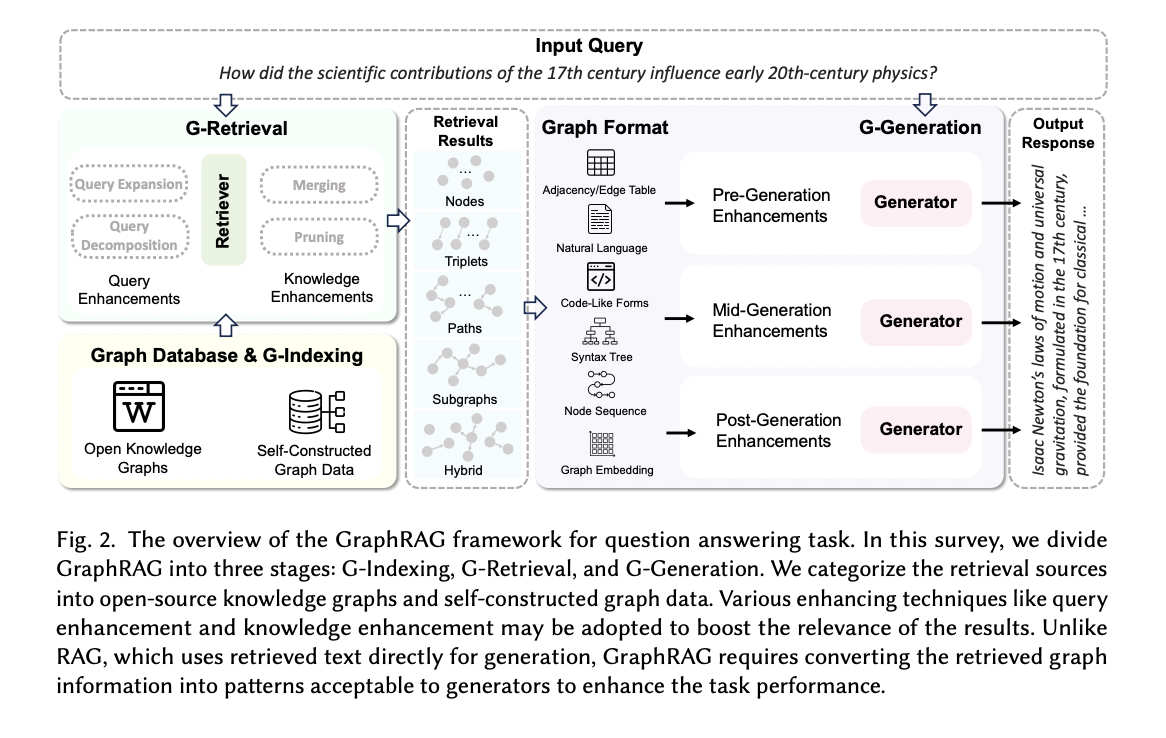
Text-Attributed Graphs (TAGs) form the foundation of GraphRAG, representing graph data with textual attributes for nodes and edges. Graph Neural Networks (GNNs) model this graph data using message-passing techniques to obtain node and graph-level representations. Language Models (LMs), both discriminative and generative, play crucial roles in GraphRAG. Initially, GraphRAG focused on improving pre-training for discriminative models. However, with the advent of LLMs like ChatGPT and LLaMA, which demonstrate powerful in-context learning capabilities, the focus has shifted to enhancing information retrieval for these models. This evolution aims to address complex tasks and mitigate hallucinations, driving rapid advancements in the field.

GraphRAG enhances language model responses by retrieving relevant knowledge from graph databases. The process involves three main stages: Graph-Based Indexing (G-Indexing), Graph-Guided Retrieval (G-Retrieval), and Graph-Enhanced Generation (G-Generation). G-Indexing creates a graph database aligned with downstream tasks. G-Retrieval extracts pertinent information from the database in response to user queries. G-Generation synthesizes outputs based on the retrieved graph data. This approach is formalized mathematically to maximize the probability of generating the optimal answer given a query and graph data. The process efficiently approximates complex graph structures to produce more informed and accurate responses.

GraphRAG’s performance heavily depends on the quality of its graph database. This foundation involves selecting or constructing appropriate graph data, ranging from open knowledge graphs to self-constructed datasets, and implementing effective indexing methods to optimize retrieval and generation processes.

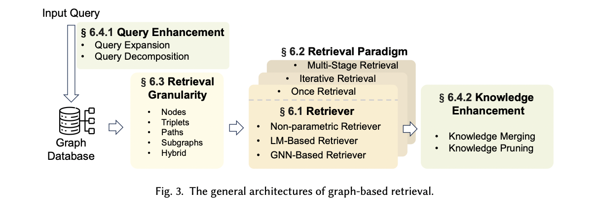
Graph data used in GraphRAG can be categorized into two main types: Open Knowledge Graphs and Self-Constructed Graph Data. Open Knowledge Graphs include General Knowledge Graphs (like Wikidata, Freebase, and DBpedia) and Domain Knowledge Graphs (such as CMeKG for biomedical fields and Wiki-Movies for the film industry). Self-Constructed Graph Data is created from various sources to meet specific task requirements. For instance, researchers have constructed document graphs, entity-relation graphs, and task-specific graphs like patent-phrase networks. The choice of graph data significantly influences GraphRAG’s performance, with each type offering unique advantages for different applications and domains.
Graph-based indexing is crucial for efficient query operations in GraphRAG, employing three main methods: graph indexing, text indexing, and vector indexing. Graph indexing preserves the entire graph structure, enabling easy access to edges and neighboring nodes. Text indexing converts graph data into textual descriptions, allowing for text-based retrieval techniques. Vector indexing transforms graph data into vector representations, facilitating rapid retrieval and efficient query processing. Each method offers unique advantages: graph indexing for structural information access, text indexing for textual content retrieval, and vector indexing for quick searches. In practice, a hybrid approach combining these methods is often preferred to optimize retrieval efficiency and effectiveness in GraphRAG systems.

The retrieval process in GraphRAG is critical for extracting relevant graph data to enhance output quality. However, it faces two major challenges: the exponential growth of candidate subgraphs as graph size increases and the difficulty in accurately measuring similarity between textual queries and graph data. To address these issues, researchers have focused on optimizing various aspects of the retrieval process. This includes developing efficient retriever models, refining retrieval paradigms, determining appropriate retrieval granularity, and implementing enhancement techniques. These efforts aim to improve the efficiency and accuracy of graph data retrieval, ultimately leading to more effective and contextually relevant outputs in GraphRAG systems.

The generation stage in GraphRAG integrates retrieved graph data with the query to produce high-quality responses. This process involves selecting appropriate generation models, transforming graph data into compatible formats, and using both the query and transformed data as inputs. Additionally, generative enhancement techniques are employed to intensify query-graph interactions and enrich content generation, further improving the final output.

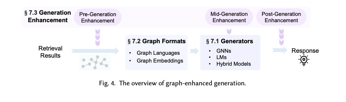
Generator selection in GraphRAG depends on the downstream task. For discriminative tasks, GNNs or discriminative language models can learn data representations and map them to answer options. Generative tasks, however, require decoders to produce text responses. While generative language models can be used for both task types, GNNs and discriminative models alone are insufficient for generative tasks that necessitate text generation.
When using LMs as generators in GraphRAG, graph translators are essential to convert non-Euclidean graph data into LM-compatible formats. This conversion process typically results in two main graph formats: graph languages and graph embeddings. These formats enable LMs to effectively process and utilize structured graph information, enhancing their generative capabilities and allowing for seamless integration of graph data in the generation process.

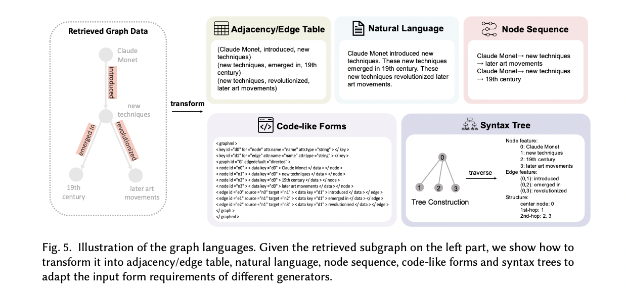
Generation enhancement techniques in GraphRAG aim to improve output quality beyond basic graph data conversion and query integration. These techniques are categorized into three stages: pre-generation, mid-generation, and post-generation enhancements. Each stage focuses on different aspects of the generation process, employing various methods to refine and optimize the final response, ultimately leading to more accurate, coherent, and contextually relevant outputs.

GraphRAG training methods are categorized into Training-Free and Training-Based approaches. Training-free methods, often used with closed-source LLMs like GPT-4, rely on carefully crafted prompts to control retrieval and generation capabilities. While utilizing LLMs’ strong text comprehension abilities, these methods may produce sub-optimal results due to a lack of task-specific optimization. Training-based methods involve fine-tuning models using supervised signals, potentially improving performance by adapting to specific task objectives. Joint training of retrievers and generators aims to enhance their synergy, boosting performance on downstream tasks. This collaborative approach utilizes the complementary strengths of both components for more robust and effective results in information retrieval and content generation applications.

GraphRAG is applied to various downstream tasks in natural language processing. These include Question Answering tasks like KBQA and CommonSense Question Answering (CSQA), which test systems’ ability to retrieve and reason over structured knowledge. Information Retrieval tasks such as Entity Linking and Relation Extraction benefit from GraphRAG’s ability to utilize graph structures. Also, GraphRAG enhances performance in fact verification, link prediction, dialogue systems, and recommender systems. In these applications, GraphRAG’s capacity to extract and analyze structured information from graphs improves accuracy, contextual relevance, and the ability to uncover latent relationships and patterns.

GraphRAG is widely applied across various domains due to its ability to integrate structured knowledge graphs with natural language processing. In e-commerce, it enhances personalized recommendations and customer service by utilizing user-product interaction graphs. In the biomedical field, it improves medical decision-making by utilizing disease-symptom-medication relationships. Academic and literature domains benefit from GraphRAG’s ability to analyze research and book relationships. In legal contexts, it aids in case analysis and legal consultation by utilizing citation networks. GraphRAG also finds applications in intelligence report generation and patent phrase similarity detection. These diverse applications demonstrate GraphRAG’s versatility in extracting and utilizing structured knowledge to enhance decision-making and information retrieval across industries.

GraphRAG systems are evaluated using two types of benchmarks: task-specific datasets and comprehensive GraphRAG-specific benchmarks like STARK, GraphQA, GRBENCH, and CRAG. Evaluation metrics fall into two categories: downstream task evaluation and retrieval quality assessment. Downstream task metrics include Exact Match, F1 score, BERT4Score, GPT4Score for KBQA, Accuracy for CSQA, and BLEU, ROUGE-L, METEOR for generative tasks. Retrieval quality is assessed using metrics such as the ratio of answer coverage to subgraph size, query relevance, diversity, and faithfulness scores. These metrics aim to provide a comprehensive evaluation of GraphRAG systems’ performance in both information retrieval and task-specific generation.

Several industrial GraphRAG systems have been developed to utilize large-scale graph data and advanced graph database technologies. Microsoft’s GraphRAG uses LLMs to construct entity-based knowledge graphs and generate community summaries for enhanced Query-Focused Summarization. NebulaGraph’s system integrates LLMs with their graph database for more precise search results. Antgroup’s framework combines DB-GPT, OpenSPG, and TuGraph for efficient triple extraction and subgraph traversal. Neo4j’s NaLLM framework explores the synergy between their graph database and LLMs, focusing on natural language interfaces and knowledge graph creation. Neo4j’s LLM Graph Builder automates knowledge graph construction from unstructured data. These systems demonstrate the growing industrial interest in combining graph technologies with large language models for enhanced performance.

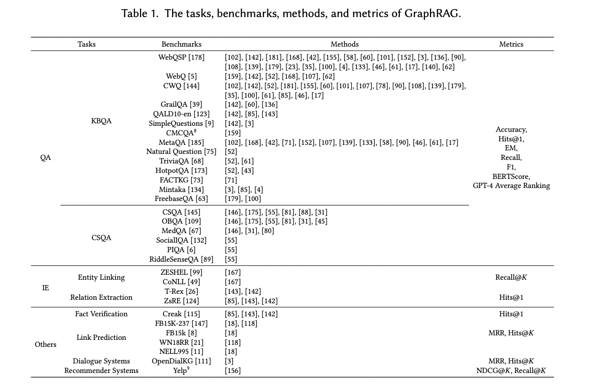
This survey provides a comprehensive overview of GraphRAG technology, systematically categorizing its fundamental techniques, training methodologies, and applications. GraphRAG enhances information retrieval by utilizing relational knowledge from graph datasets, addressing the limitations of traditional RAG approaches. As a nascent field, the survey outlines benchmarks, analyzes current challenges, and illuminates future research directions. This comprehensive analysis offers valuable insights into GraphRAG’s potential to improve the relevance, accuracy, and comprehensiveness of information retrieval and generation systems.

Check out the Paper . All credit for this research goes to the researchers of this project. Also, don’t forget to follow us on Twitter and join our Telegram Channel and LinkedIn Gr oup . If you like our work, you will love our newsletter..

Don’t Forget to join our 49k+ ML SubReddit

Find Upcoming AI Webinars here

Mohammad Asjad

Asjad is an intern consultant at Marktechpost. He is persuing B.Tech in mechanical engineering at the Indian Institute of Technology, Kharagpur. Asjad is a Machine learning and deep learning enthusiast who is always researching the applications of machine learning in healthcare.

Jina AI Introduced 'Late Chunking': A Simple AI Approach to Embed Short Chunks by Leveraging the Power of Long-Context Embedding Models
Humboldt: A Specification-based System Framework for Generating a Data Discovery UI from Different Metadata Providers
Improving RLHF (Reinforcement Learning from Human Feedback) with Critique-Generated Reward Models
AWS Enhancing Information Retrieval in Large Language Models: A Data-Centric Approach Using Metadata, Synthetic QAs, and Meta Knowledge Summaries for Improved Accuracy and Relevancy

Privacy Overview

IMAGES

Sensors
(PDF) Graph Representation Learning and Its Applications: A Survey
Sensors
(PDF) Graph representation learning: a survey
Representation Learning in Knowledge Graphs
Graph Representation Learning: A Survey

VIDEO

Yusu Wang
The Distributed Open Source Graph Database
Graph Representation in Data Structure |Adjacency Matrix and Adjacecy List
[tt8745] Text-Attributed Graph Representation Learning: Methods, Applications, and Challenges
A Survey of Text Representation and Embedding Techniques in NLP
Lesson 2.1 Stem-and-Leaf Graphs, Line Graphs, and Bar Charts

COMMENTS

Graph Representation Learning and Its Applications: A Survey
Graphs are data structures that effectively represent relational data in the real world. Graph representation learning is a significant task since it could facilitate various downstream tasks, such as node classification, link prediction, etc. Graph representation learning aims to map graph entities to low-dimensional vectors while preserving graph structure and entity relationships. Over the ...
Graph Representation Learning and Its Applications: A Survey
Graph representation learning is a significant task since it could facilitate various downstream tasks, such as node classification, link prediction, etc. Graph representation learning aims to map graph entities to low-dimensional vectors while preserving graph structure and entity relationships. Over the decades, many models have been proposed ...
[1909.00958] Graph Representation Learning: A Survey
View a PDF of the paper titled Graph Representation Learning: A Survey, by Fenxiao Chen and 2 other authors. Research on graph representation learning has received a lot of attention in recent years since many data in real-world applications come in form of graphs. High-dimensional graph data are often in irregular form, which makes them more ...
Graph Representation Learning and Its Applications: A Survey
Abstract: Graphs are data structures that effectively repr esent relational data in the real world. Graph. representation learning is a signiﬁcant task since it could facilitate various ...
Graph Representation Learning and Its Applications: A Survey.
2. Problem Description. Graph representation learning aims to project the graph entities into low-dimensional vectors while preserving the graph structure and the proximity of entities in graphs. With the desire to map graph entities into vector space, it is necessary to model the graph in mathematical form.
Graph Representation Learning and Its Applications: A Survey
Graph Representation Learning and Its Applications: A Survey. This paper aims to show a comprehensive picture of graph representation learning models, including traditional and state-of-the-art models on various graphs in different geometric spaces, and provides a structured overview of the diversity of graph embedding models.
PDF Graph Representation Learning and Its Applications: A Survey
Graph Representation Learning and Its Applications: A Survey Van Thuy Hoang 1, Hyeon-Ju Jeon 2, Eun-Soon You 1, Yoewon Yoon 3, Sungyeop Jung 4, and O-Joun Lee 1,* 1 Department of Artiﬁcial Intelligence, The Catholic University of Korea, 43, Jibong-ro, Bucheon-si 14662, Gyeonggi-do, Republic of Korea; [email protected] (V.T.H.);
A Comprehensive Survey on Deep Graph Representation Learning
Specifically, we systematically summarize the essential components of graph representation learning and categorize existing approaches by the ways of graph neural network architectures and the most recent advanced learning paradigms. Moreover, this survey also provides the practical and promising applications of deep graph representation learning.
A Comprehensive Survey on Deep Graph Representation Learning
Graph representation learning aims to effectively encode high-dimensional sparse graph-structured data into low-dimensional dense vectors, which is a fundamental task that has been widely studied in a range of fields, including machine learning and data mining. Classic graph embedding methods follow the basic idea that the embedding vectors of interconnected nodes in the graph can still ...
Graph Representation Learning Meets Computer Vision: A Survey
A graph structure is a powerful mathematical abstraction, which can not only represent information about individuals but also capture the interactions between individuals for reasoning. Geometric modeling and relational inference based on graph data is a long-standing topic of interest in the computer vision community. In this article, we provide a systematic review of graph representation ...
[2204.01855] A Survey on Graph Representation Learning Methods
In this survey, we provide an overview of these two categories and cover the current state-of-the-art methods for both static and dynamic graphs. Finally, we explore some open and ongoing research directions for future work. Subjects: Machine Learning (cs.LG); Social and Information Networks (cs.SI) Cite as: arXiv:2204.01855 [cs.LG]
[PDF] Graph representation learning: a survey
This review reviews a wide range of graph embedding techniques with insights and evaluates several stat-of-the-art methods against small and large data sets and compare their performance. Abstract Research on graph representation learning has received great attention in recent years since most data in real-world applications come in the form of graphs. High-dimensional graph data are often in ...
(PDF) Graph representation learning: a survey
Abstract and Figures. Research on graph representation learning has received great attention in recent years since most data in real-world applications come in the form of graphs. High-dimensional ...
now publishers
Research on graph representation learning has received great attention in recent years since most data in real-world applications come in the form of graphs. High-dimensional graph data are often in irregular forms. They are more difficult to analyze than image/video/audio data defined on regular lattices. Various graph embedding techniques ...
Graph Representation Learning and Its Applications: A Survey
Historically, the first graph representation learning models were graph kernels. The idea of graph kernel methods perhaps comes from the most essential and well-known Weisfeiler-Lehman (WL) isomorphic testing in 1968 [].Graph kernels are kernel functions that aim to measure the similarity between graphs and their entities [].The main idea of graph kernels is to decompose original graphs into ...
Graph Representation Learning Meets Computer Vision: A Survey
The evolution of representation learning on graphs is sort out into the nonneural network and neural network methods based on the way the nodes are encoded, and the existing challenges and future directions of graph representation learning and computer vision are discussed. A graph structure is a powerful mathematical abstraction, which can not only represent information about individuals but ...
Graph representation learning in biomedicine and healthcare
Graph representation learning exploits relational inductive biases for data that come in the form of graphs. In some settings, however, the graphs are not readily available for learning. This is ...
Graph representation learning for popularity prediction problem: A survey
A lot of efforts have been focused on this problem to help us better understand and achieve higher performance in viral marketing and advertising. On the other hand, the development of neural networks has blossomed in the last few years, leading to a large number of graph representation learning (GRL) models.
A Survey of Large Language Models for Graphs
Integrating LLMs with graph learning techniques has attracted interest as a way to enhance performance in graph learning tasks. In this survey, we conduct an in-depth review of the latest state-of-the-art LLMs applied in graph learning and introduce a novel taxonomy to categorize existing methods based on their framework design.
Enhanced Knowledge Graph Attention Networks for Efficient Graph
This paper introduces an innovative design for Enhanced Knowledge Graph Attention Networks (EKGAT), focusing on improving representation learning for graph-structured data. By integrating TransformerConv layers, the proposed EKGAT model excels in capturing complex node relationships compared to traditional KGAT models. Additionally, our EKGAT model integrates disentanglement learning ...
[2212.08966] Graph Learning and Its Advancements on Large Language
View a PDF of the paper titled Graph Learning and Its Advancements on Large Language Models: A Holistic Survey, by Shaopeng Wei and 7 other authors. Graph learning is a prevalent domain that endeavors to learn the intricate relationships among nodes and the topological structure of graphs. Over the years, graph learning has transcended from ...
SiSRS: Signed social recommender system using deep neural network
A comprehensive survey on graph neural networks. IEEE Transactions on Neural Networks and Learning Systems, 32 (1) (2020) ... Deep Representation Learning using Multilayer Perceptron and Stacked Autoencoder for Recommendation Systems. ... Statistical Mechanics and its Applications, 520 (2019), pp. 317-321. View PDF View article View in Scopus ...
PDF Graph Representation Learning and Its Applications: A Survey
Sensors 2023, 23, 4168 3 of 105 Historically, the ﬁrst graph representation learning models were graph kernels. The idea of graph kernel methods perhaps comes from the most essential and well-known
Graph Representation and Anonymization in Large Survey Rating Data
Graph Representation and Anonymization in Large Survey Rating Data: 10.4018/978-1-61350-053-8.ch014: We study the challenges of protecting privacy of individuals in the large public survey rating data in this chapter. Recent study shows that personal. Get IGI Global News;
Document-Level Event Argument Extraction with Sparse Representation
Document-level Event Argument Extraction (DEAE) aims to extract structural event knowledge composed of arguments and roles beyond the sentence level. Existing methods mainly focus on designing prompts and using Abstract Meaning Representation (AMR) graph structure as additional features to enrich event argument representation. However, two challenges still remain: (1) the long-range dependency ...
Graph Fourier transform for spatial omics representation and ...
Within this representation of FTUs, a binary graph signal (e.g., 0,1), representing discrete two-state information at each node, and cellular or subcellular composition or omics features (e.g ...
Graph Retrieval-Augmented Generation: A Survey
Knowledge Graph Reasoning. In The Twelfth International Conference on Learning Representations. [35] Hanning Gao, Lingfei Wu, Po Hu, Zhihua Wei, Fangli Xu, and Bo Long. 2022. Graph-augmented Learning to Rank for Querying Large-scale Knowledge Graph. In Proceedings of the 2nd Conference of the Asia-Pacific Chapter of the
Integrating Graph Structures into Language Models: A Comprehensive
This survey provides a comprehensive overview of GraphRAG technology, systematically categorizing its fundamental techniques, training methodologies, and applications. GraphRAG enhances information retrieval by utilizing relational knowledge from graph datasets, addressing the limitations of traditional RAG approaches.
Deep learning of multimodal networks with topological regularization
Computational techniques for drug-disease prediction are essential in enhancing drug discovery and repositioning. While many methods utilize multimodal networks from various biological databases, few integrate comprehensive multi-omics data, including transcriptomes, proteomes, and metabolomes. We introduce STRGNN, a novel graph deep learning approach that predicts drug-disease relationships ...

Save citation to file

Add to My Bibliography

Graph Representation Learning and Its Applications: A Survey

Conflict of interest statement

Similar articles

Publication types

Grants and funding

LinkOut - more resources

Research Materials

IEEE Account

Purchase Details

Profile Information

Export citation

Graph representation learning: a survey

Graph Representation Learning and Its Applications: A Survey

Hyeon-Ju Jeon

Eun-Soon You

Sungyeop Jung

Associated Data

1. Introduction

2. Problem Description

3. Graph Representation Learning Models

3.1. Graph Kernels

3.2. Matrix Factorization-Based Models

3.3. Shallow Models

3.3.1. Structure-Preservation Models

3.3.2. Proximity Reconstruction Models

3.4. Deep Neural Network-Based Models

3.4.1. Graph Autoencoders

3.4.2. Recurrent Graph Neural Networks

3.4.3. Convolutional Graph Neural Networks

3.4.4. Graph Transformer Models

3.5. Non-Euclidean Models

3.5.1. Hyperbolic Embedding Models

3.5.2. Spherical Embedding Models

3.5.3. Gaussian Embedding Models

4. Applications

4.1. Computer Vision

4.2. Natural Language Processing

4.3. Computer Security

4.4. Bioinformatics

4.5. Social Media Analysis

4.6. Recommendation Systems

4.7. Smart Cities

4.8. Computational Social Science

4.9. Digital Humanity

4.10. Semiconductor Manufacturing

4.11. Weather Forecasting

5. Evaluation Methods

5.1. Benchmark Datasets

5.2. Downstream Tasks and Evaluation Metrics

5.3. Libraries for Graph Representation Learning

6. Challenges and Future Research Directions

7. Conclusions

Appendix A. Open-Source Implementations

Funding Statement

Author Contributions

Institutional Review Board Statement

Informed Consent Statement

Graph Representation Learning Meets Computer Vision: A Survey

Figures and Tables from this paper

36 Citations

How Powerful are Graph Neural Networks?

Login to your account

Password Changed Successfully

Create a new account

Request Username

Cookies Notification

Adblock Instructions

uBlock Origin Instructions

uBlock Instructions

Adguard Instructions

Brave Instructions

Adremover Instructions

Adblock Genesis Instructions

Super Adblocker Instructions

Ultrablock Instructions

Ad Aware Instructions

Ghostery Instructions

Firefox Tracking Protection Instructions